ECE 275: Multi-output functions
Website: https://vikasdhiman.info/ECE275-Sequential-Logic/
\[
\newcommand{\bx}{\bar{x}}
\newcommand{\by}{\bar{y}}
\newcommand{\bz}{\bar{z}}
\]
Announcments
- Homework 3 is due on Sept 27th, Monday before class.
Limitations of this course
- For 2-5 variables use K-Map
- For upto 15 variables, use Quine McCluskey method (NP complete). Complexity grows exponentially with number of input variables
- EXPRESSO-Exact, EXPRESSO-II, CAPPUCCINO are a few of the popular methods that are taught in advanced version of this course.
Multi output functions: Ex 1
\( f_1 \)
| \(\bar{x}_1\) | \(x_1 \) | ||||
|---|---|---|---|---|---|
| \(\bar{x}_2\) | \(x_2 \) | \(\bar{x}_2\) | |||
| \(\bar{x}_3\) | \(\bar{x}_4\) | 0 | 0 | 0 | 0 |
| \(x_4\) | 0 | 1 | 1 | 0 | |
| \(x_3\) | 0 | 1 | 1 | 0 | |
| \(\bar{x}_4\) | 1 | 1 | 0 | 0 | |
\( f_2 \)
| \(\bar{x}_1\) | \(x_1 \) | ||||
|---|---|---|---|---|---|
| \(\bar{x}_2\) | \(x_2 \) | \(\bar{x}_2\) | |||
| \(\bar{x}_3\) | \(\bar{x}_4\) | 0 | 0 | 0 | 0 |
| \(x_4\) | 0 | 1 | 0 | 0 | |
| \(x_3\) | 0 | 1 | 0 | 0 | |
| \(\bar{x}_4\) | 1 | 1 | 0 | 0 | |
\( f_3 \)
| \(\bar{x}_1\) | \(x_1 \) | ||||
|---|---|---|---|---|---|
| \(\bar{x}_2\) | \(x_2 \) | \(\bar{x}_2\) | |||
| \(\bar{x}_3\) | \(\bar{x}_4\) | 0 | 0 | 0 | 0 |
| \(x_4\) | 0 | 0 | 1 | 1 | |
| \(x_3\) | 0 | 0 | 1 | 0 | |
| \(\bar{x}_4\) | 0 | 0 | 0 | 0 | |
Ex 1: Soln
Separately optimized
\( g_1 = \bx_1 x_3 \bx_4 \), Cost = 1 + 3 = 4\( f_1 = x_2 x_4 + g_1 \), Cost = 1 + 1 + 2 + 2 = 6
\( f_2 = \bx_1 x_2 x_4 + g_1 \), Cost = 1 + 1 + 3 + 2= 7
\( f_3 = x_1 x_2 x_4 + x_1 \bx_3 x_4 \), Cost = 2 + 1 + 3 + 3 + 2 = 11
Total Cost: 28
Jointly optimized
\( g_1 = \bx_1 x_3 \bx_4 \), Cost = 1 + 3 = 4\( g_2 = x_1 x_2 x_4 \), Cost = 1 + 3 = 4
\( g_3 = \bx_1 x_2 x_4 \), Cost = 1 + 3 = 4
\( f_1 = g_1 + g_2 + g_3 \), Cost = 1 + 3 = 4
\( f_2 = g_3 + g_1 \), Cost = 1 + 2 = 3
\( f_3 = g_2 + x_1 \bx_3 x_4 \), Cost = 1 + 1 + 3 + 2 = 7
Total Cost: 26
Multi output functions: Ex 2
\( f_1 \)
| \(\bar{x}_1\) | \(x_1 \) | ||||
|---|---|---|---|---|---|
| \(\bar{x}_2\) | \(x_2 \) | \(\bar{x}_2\) | |||
| \(\bar{x}_3\) | \(\bar{x}_4\) | 0 | 0 | 1 | 0 |
| \(x_4\) | 0 | 0 | 1 | 0 | |
| \(x_3\) | 0 | 0 | 1 | 1 | |
| \(\bar{x}_4\) | 0 | 0 | 1 | 0 | |
\( f_2 \)
| \(\bar{x}_1\) | \(x_1 \) | ||||
|---|---|---|---|---|---|
| \(\bar{x}_2\) | \(x_2 \) | \(\bar{x}_2\) | |||
| \(\bar{x}_3\) | \(\bar{x}_4\) | 0 | 0 | 1 | 0 |
| \(x_4\) | 0 | 0 | 1 | 0 | |
| \(x_3\) | 1 | 1 | 1 | 1 | |
| \(\bar{x}_4\) | 0 | 0 | 0 | 0 | |
\( f_3 \)
| \(\bar{x}_1\) | \(x_1 \) | ||||
|---|---|---|---|---|---|
| \(\bar{x}_2\) | \(x_2 \) | \(\bar{x}_2\) | |||
| \(\bar{x}_3\) | \(\bar{x}_4\) | 0 | 0 | 1 | 0 |
| \(x_4\) | 1 | 1 | 1 | 0 | |
| \(x_3\) | 0 | 0 | 1 | 0 | |
| \(\bar{x}_4\) | 0 | 0 | 1 | 0 | |
Ex 3
\( f_1 \)
| \(\bar{x}_1\) | \(x_1 \) | ||||
|---|---|---|---|---|---|
| \(\bar{x}_2\) | \(x_2 \) | \(\bar{x}_2\) | |||
| \(\bar{x}_3\) | \(\bar{x}_4\) | 0 | 0 | 1 | 0 |
| \(x_4\) | 0 | 0 | 1 | 0 | |
| \(x_3\) | 0 | 0 | 1 | 1 | |
| \(\bar{x}_4\) | 0 | 0 | 1 | 0 | |
\( f_2 \)
| \(\bar{x}_1\) | \(x_1 \) | ||||
|---|---|---|---|---|---|
| \(\bar{x}_2\) | \(x_2 \) | \(\bar{x}_2\) | |||
| \(\bar{x}_3\) | \(\bar{x}_4\) | 0 | 0 | 1 | 0 |
| \(x_4\) | 0 | 0 | 1 | 0 | |
| \(x_3\) | 1 | 1 | 1 | 1 | |
| \(\bar{x}_4\) | 0 | 0 | 0 | 0 | |
\( f_3 \)
| \(\bar{x}_1\) | \(x_1 \) | ||||
|---|---|---|---|---|---|
| \(\bar{x}_2\) | \(x_2 \) | \(\bar{x}_2\) | |||
| \(\bar{x}_3\) | \(\bar{x}_4\) | 0 | 0 | 1 | 0 |
| \(x_4\) | 0 | 0 | 1 | 0 | |
| \(x_3\) | 1 | 1 | 1 | 0 | |
| \(\bar{x}_4\) | 0 | 0 | 1 | 0 | |

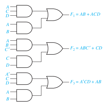
\[ F_1 = AB + ACD \]
\[ F_2 = AB\bar{C} + \bar{A}CD + ACD \]
\[ F_3 = AB + \bar{A}CD \]
EPIs for Multi-output functions
For multiple output functions, we consider only those 1's for EPI that are not present in other fuction maps.
\( f_1 \)
| \(\bar{x}_1\) | \(x_1 \) | ||||
|---|---|---|---|---|---|
| \(\bar{x}_2\) | \(x_2 \) | \(\bar{x}_2\) | |||
| \(\bar{x}_3\) | \(\bar{x}_4\) | 0 | 0 | 0 | 0 |
| \(x_4\) | 1 | 1 | 1 | 1 | |
| \(x_3\) | 0 | 0 | 1 | 0 | |
| \(\bar{x}_4\) | 0 | 0 | 0 | 0 | |
\( f_2 \)
| \(\bar{x}_1\) | \(x_1 \) | ||||
|---|---|---|---|---|---|
| \(\bar{x}_2\) | \(x_2 \) | \(\bar{x}_2\) | |||
| \(\bar{x}_3\) | \(\bar{x}_4\) | 0 | 1 | 1 | 0 |
| \(x_4\) | 0 | 0 | 0 | 0 | |
| \(x_3\) | 0 | 0 | 1 | 0 | |
| \(\bar{x}_4\) | 0 | 1 | 1 | 0 | |
Limitations of this course
- Quine McCluskey can be extended to Multi-output functions: http://web.mit.edu/6.111/www/f2017/handouts/qm.pdf
Propagation Delay

Hazards
Hazards: Example
Hazards: Example fixed
To avoid static hazards, "close all the gaps" in the K-map by adding extra product terms (or sum terms for POS).
- SOP can only have static-1 hazards.
- POS can only have static-0 hazards.
- More than 2-level circuits needed for dynamic hazards.
Thanks, Questions, Feedback?
https://vikasdhiman.info/ECE275-Sequential-Logic/