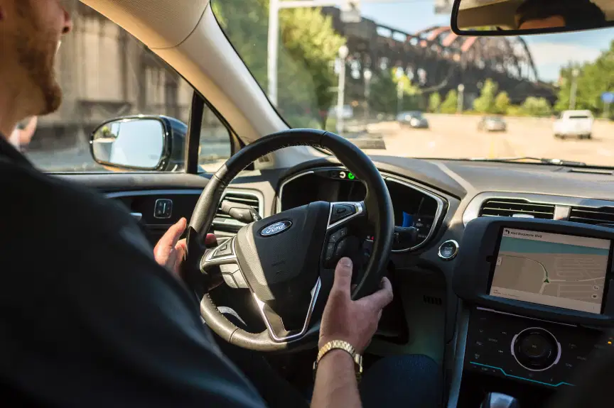
Autonomous driving and safety

\( \newcommand{\TODO}[1]{{\color{red}TODO: {#1}}} \renewcommand{\vec}[1]{\mathbf{#1}} \newcommand{\state}{\vec{x}} \def\statet{\state_t} \def\statetp{\state_{t-1}} \def\statehist{\state_{1:t-1}} \def\statetn{\state_{t+1}} \def\obs{\meas} \def\obst{\obs_t} \def\act{a} \def\actt{\act_t} \def\acttp{\act_{t-1}} \def\acttn{\act_{t+1}} \def\Obs{\mathcal{O}} \def\ObsEnc{\Phi_o} \def\ObsProb{P_o} \def\ObsFunc{C} \def\ObsFuncFull{\ObsFunc(\statet, \actt) \rightarrow \obst} \def\ObsFuncInv{\ObsFunc^{-1}} \def\ObsFuncInvFull{\ObsFuncInv(\obst, \statetp, \actt) \rightarrow \statet} \def\StateSp{\mathcal{X}} \def\Action{\mathcal{A}} \def\TransP{P_{T}} \def\Trans{T} \def\TransFull{\Trans(\statet, \actt) \rightarrow \statetn} \def\TransObs{T_c} \def\Rew{R} \def\rew{r} \def\rewards{\vec{r}_{1:t}} \def\rewt{\rew_t} \def\rewtp{\rew_{t-1}} \def\rewtn{\rew_{t+1}} \def\RewFull{\Rew(\statet, \actt) \rightarrow \rewtn} \def\TransObsFull{\TransObs(\statet, \obst, \actt, \rewt; \theta_T) \rightarrow \statetn} \def\Value{V} \def\pit{\pi_t} \def\piDef{\pi(\acttn|\statet, \obst, \actt, \rewt; \theta_\pi) \rightarrow \pit(\acttn ; \theta_\pi)} \def\Valuet{\Value_t} \def\ValueDef{\Value(\statet, \obst, \actt, \rewt; \theta_\Value) \rightarrow \Valuet(\theta_\Value)} \def\R{\mathbb{R}} \def\E{\mathbb{E}} \newcommand{\Goal}{\mathcal{G}} \newcommand{\goalRV}{G} \newcommand{\meas}{z} \newcommand{\measurements}{\vec{\meas}_{1:t}} \newcommand{\meast}[1][t]{\meas_{#1}} \newcommand{\param}{\theta} \newcommand{\policy}{\pi} \newcommand{\graph}{G} \newcommand{\vtces}{V} \newcommand{\edges}{E} \newcommand{\st}{\state} \newcommand{\stn}{\st_{t+1}} \newcommand{\stt}{\st_t} \newcommand{\stk}{\st_k} \newcommand{\stj}{\st_j} \newcommand{\sti}{\st_i} \newcommand{\St}{\mathcal{S}} \newcommand{\Act}{\mathcal{A}} \newcommand{\acti}{\act_i} \newcommand{\lpt}{\delta} \newcommand{\trans}{P_T} \newcommand{\Q}{\qValue} \newcommand{\fwcost}{Q} \newcommand{\fw}{\fwcost} \newcommand{\qValue}{Q} \newcommand{\prew}{\Upsilon} \newcommand{\epiT}{T} \newcommand{\vma}{\alpha_\Value} \newcommand{\qma}{\alpha_\qValue} \newcommand{\prewma}{\alpha_\prew} \newcommand{\fwma}{\alpha_\fwcost} \newcommand{\maxValueBeam}{\vec{\state}_{\Value:\text{max}(m)}} \newcommand{\nil}{\emptyset} \newcommand{\discount}{\gamma} \newcommand{\minedgecost}{\fwcost_0} \newcommand{\goal}{g} \newcommand{\pos}{x} %\newcommand{\fwargs}[5]{\fw_{#4}^{#5}\left({#3}\middle|{#1}, {#2}\right)} \newcommand{\fwargs}[5]{\fw_{#4}^{#5}\left({#1}, {#2}, {#3}\right)} \newcommand{\Rgoal}{R_{\text{goal}}} \newcommand{\Loo}{Latency-1:\textgreater1} \newcommand{\Loss}{\mathcal{L}} \newcommand{\LossText}[1]{\Loss_{\text{#1}}} \newcommand{\LossDDPG}{\LossText{ddpg}} \newcommand{\LossStep}{\LossText{step}} \newcommand{\LossLo}{\LossText{lo}} \newcommand{\LossUp}{\LossText{up}} \newcommand{\LossTrieq}{\LossText{trieq}} \newcommand{\tgt}{\text{tgt}} \newcommand{\Qstar}{\Q_{*}} \newcommand{\Qtgt}{\Q_{\text{tgt}}} \newcommand{\ytgt}{y_t} % Symbols \newcommand{\ctrl}{\vec{u}} \newcommand{\Ctrl}{\mathcal{U}} \newcommand{\Data}{\mathcal{D}} \newcommand{\stdt}{\dot{\state}} \newcommand{\StDt}{\dot{\StateSp}} \newcommand{\dynSt}{f} \newcommand{\dynCt}{g} \newcommand{\bDynSt}{\bar{\dynSt}} \newcommand{\bDynCt}{\bar{\dynCt}} \newcommand{\dynAff}{F} \newcommand{\bDynAff}{\bar{\dynAff}} \newcommand{\ctrlaff}{\underline{\mathbf{\ctrl}}} \newcommand{\smallbmat}[1]{\left[\begin{smallmatrix}#1\end{smallmatrix}\right]} \newcommand{\Knl}{K} \newcommand{\knl}{\kappa} \newcommand{\bKx}{k_\state} \newcommand{\bKF}{k_\dynAff} \newcommand{\bKFu}{k_{\dynAff\ctrl}} \newcommand{\bKFx}{k_{\dynAff\state}} \newcommand{\bKFux}{k_{\dynAff\ctrl\state}} \newcommand{\covf}{\text{cov}} \newcommand{\dt}{\delta t} \newcommand{\dSt}{\stdt} \newcommand{\N}{\mathcal{N}} \newcommand{\StDat}{\mathbf{X}} \newcommand{\StDtDat}{\dot{\mathbf{X}}} \newcommand{\CtDat}{\underline{\boldsymbol{\mathcal{U}}}_{1:k}} \newcommand{\mat}[1]{{#1}} \newcommand{\Y}{\mat{Y}} \newcommand{\bY}{\bar{\Y}} \newcommand{\W}{\mat{W}} \newcommand{\V}{\mat{V}} \newcommand{\mH}{\mat{H}} \newcommand{\KH}{\Knl^\mH} \newcommand{\kH}{\knl^\mH} \newcommand{\GP}{\mathcal{GP}} \newcommand{\kDA}{\knl^\dynAff} \newcommand{\KDA}{\Knl^\dynAff} %\newcommand{\M}{\mathcal{M}} \newcommand{\kh}{\knl^{\dynAff\ctrlaff}} \newcommand{\KDat}{\mathfrak{K}} \newcommand{\kDat}{\bm{\knl}} \newcommand{\KhDat}{\KDat^{\dynAff\ctrlaff}} \newcommand{\khDADat}{\kDat^{\dynAff\ctrlaff\dynAff}} \newcommand{\khDA}{\knl^{\dynAff\ctrlaff\dynAff}} \newcommand{\dynAffDat}{\mathbf{\dynAff}} \newcommand{\grad}{\nabla} \newcommand{\Lie}{\mathcal{L}} \newcommand{\tdf}{\tilde{f}} \newcommand{\tdg}{\tilde{g}} \newcommand{\barf}{\bar{f}} \newcommand{\barg}{\bar{g}} \newcommand{\erf}{\textit{erf}} \newcommand{\etal}{et~al.} \newcommand{\CBC}{\mbox{CBC}} \newcommand{\CBCtwo}{\CBC^{(2)}} \newcommand{\CBCr}{\CBC^{(r)}} \newcommand{\Prob}{\mathbb{P}} \newcommand{\tdbff}{\bff^*_k} \newcommand{\mDynAffs}{\bfM_k} \newcommand{\bfBs}{\bfB_k} \DeclareMathOperator{\vect}{\textit{vec}} \DeclareMathOperator{\diag}{\mathbf{diag}} \DeclareMathOperator{\cov}{cov} \DeclareMathOperator{\Cov}{\mathbf{Cov}} \DeclareMathOperator{\Var}{Var} % Calligraphic fonts \newcommand{\calA}{{\cal A}} \newcommand{\calB}{{\cal B}} \newcommand{\calC}{{\cal C}} \newcommand{\calD}{{\cal D}} \newcommand{\calE}{{\cal E}} \newcommand{\calF}{{\cal F}} \newcommand{\calG}{{\cal G}} \newcommand{\calH}{{\cal H}} \newcommand{\calI}{{\cal I}} \newcommand{\calJ}{{\cal J}} \newcommand{\calK}{{\cal K}} \newcommand{\calL}{{\cal L}} \newcommand{\calM}{{\cal M}} \newcommand{\calN}{{\cal N}} \newcommand{\calO}{{\cal O}} \newcommand{\calP}{{\cal P}} \newcommand{\calQ}{{\cal Q}} \newcommand{\calR}{{\cal R}} \newcommand{\calS}{{\cal S}} \newcommand{\calT}{{\cal T}} \newcommand{\calU}{{\cal U}} \newcommand{\calV}{{\cal V}} \newcommand{\calW}{{\cal W}} \newcommand{\calX}{{\cal X}} \newcommand{\calY}{{\cal Y}} \newcommand{\calZ}{{\cal Z}} % Sets: \newcommand{\setA}{\textsf{A}} \newcommand{\setB}{\textsf{B}} \newcommand{\setC}{\textsf{C}} \newcommand{\setD}{\textsf{D}} \newcommand{\setE}{\textsf{E}} \newcommand{\setF}{\textsf{F}} \newcommand{\setG}{\textsf{G}} \newcommand{\setH}{\textsf{H}} \newcommand{\setI}{\textsf{I}} \newcommand{\setJ}{\textsf{J}} \newcommand{\setK}{\textsf{K}} \newcommand{\setL}{\textsf{L}} \newcommand{\setM}{\textsf{M}} \newcommand{\setN}{\textsf{N}} \newcommand{\setO}{\textsf{O}} \newcommand{\setP}{\textsf{P}} \newcommand{\setQ}{\textsf{Q}} \newcommand{\setR}{\textsf{R}} \newcommand{\setS}{\textsf{S}} \newcommand{\setT}{\textsf{T}} \newcommand{\setU}{\textsf{U}} \newcommand{\setV}{\textsf{V}} \newcommand{\setW}{\textsf{W}} \newcommand{\setX}{\textsf{X}} \newcommand{\setY}{\textsf{Y}} \newcommand{\setZ}{\textsf{Z}} % Vectors \newcommand{\bfa}{\mathbf{a}} \newcommand{\bfb}{\mathbf{b}} \newcommand{\bfc}{\mathbf{c}} \newcommand{\bfd}{\mathbf{d}} \newcommand{\bfe}{\mathbf{e}} \newcommand{\bff}{\mathbf{f}} \newcommand{\bfg}{\mathbf{g}} \newcommand{\bfh}{\mathbf{h}} \newcommand{\bfi}{\mathbf{i}} \newcommand{\bfj}{\mathbf{j}} \newcommand{\bfk}{\mathbf{k}} \newcommand{\bfl}{\mathbf{l}} \newcommand{\bfm}{\mathbf{m}} \newcommand{\bfn}{\mathbf{n}} \newcommand{\bfo}{\mathbf{o}} \newcommand{\bfp}{\mathbf{p}} \newcommand{\bfq}{\mathbf{q}} \newcommand{\bfr}{\mathbf{r}} \newcommand{\bfs}{\mathbf{s}} \newcommand{\bft}{\mathbf{t}} \newcommand{\bfu}{\mathbf{u}} \newcommand{\bfv}{\mathbf{v}} \newcommand{\bfw}{\mathbf{w}} \newcommand{\bfx}{\mathbf{x}} \newcommand{\bfy}{\mathbf{y}} \newcommand{\bfz}{\mathbf{z}} \newcommand{\bfalpha}{\boldsymbol{\alpha}} \newcommand{\bfbeta}{\boldsymbol{\beta}} \newcommand{\bfgamma}{\boldsymbol{\gamma}} \newcommand{\bfdelta}{\boldsymbol{\delta}} \newcommand{\bfepsilon}{\boldsymbol{\epsilon}} \newcommand{\bfzeta}{\boldsymbol{\zeta}} \newcommand{\bfeta}{\boldsymbol{\eta}} \newcommand{\bftheta}{\boldsymbol{\theta}} \newcommand{\bfiota}{\boldsymbol{\iota}} \newcommand{\bfkappa}{\boldsymbol{\kappa}} \newcommand{\bflambda}{\boldsymbol{\lambda}} \newcommand{\bfmu}{\boldsymbol{\mu}} \newcommand{\bfnu}{\boldsymbol{\nu}} \newcommand{\bfomicron}{\boldsymbol{\omicron}} \newcommand{\bfpi}{\boldsymbol{\pi}} \newcommand{\bfrho}{\boldsymbol{\rho}} \newcommand{\bfsigma}{\boldsymbol{\sigma}} \newcommand{\bftau}{\boldsymbol{\tau}} \newcommand{\bfupsilon}{\boldsymbol{\upsilon}} \newcommand{\bfphi}{\boldsymbol{\phi}} \newcommand{\bfchi}{\boldsymbol{\chi}} \newcommand{\bfpsi}{\boldsymbol{\psi}} \newcommand{\bfomega}{\boldsymbol{\omega}} \newcommand{\bfxi}{\boldsymbol{\xi}} \newcommand{\bfell}{\boldsymbol{\ell}} % Matrices \newcommand{\bfA}{\mathbf{A}} \newcommand{\bfB}{\mathbf{B}} \newcommand{\bfC}{\mathbf{C}} \newcommand{\bfD}{\mathbf{D}} \newcommand{\bfE}{\mathbf{E}} \newcommand{\bfF}{\mathbf{F}} \newcommand{\bfG}{\mathbf{G}} \newcommand{\bfH}{\mathbf{H}} \newcommand{\bfI}{\mathbf{I}} \newcommand{\bfJ}{\mathbf{J}} \newcommand{\bfK}{\mathbf{K}} \newcommand{\bfL}{\mathbf{L}} \newcommand{\bfM}{\mathbf{M}} \newcommand{\bfN}{\mathbf{N}} \newcommand{\bfO}{\mathbf{O}} \newcommand{\bfP}{\mathbf{P}} \newcommand{\bfQ}{\mathbf{Q}} \newcommand{\bfR}{\mathbf{R}} \newcommand{\bfS}{\mathbf{S}} \newcommand{\bfT}{\mathbf{T}} \newcommand{\bfU}{\mathbf{U}} \newcommand{\bfV}{\mathbf{V}} \newcommand{\bfW}{\mathbf{W}} \newcommand{\bfX}{\mathbf{X}} \newcommand{\bfY}{\mathbf{Y}} \newcommand{\bfZ}{\mathbf{Z}} \newcommand{\bfGamma}{\boldsymbol{\Gamma}} \newcommand{\bfDelta}{\boldsymbol{\Delta}} \newcommand{\bfTheta}{\boldsymbol{\Theta}} \newcommand{\bfLambda}{\boldsymbol{\Lambda}} \newcommand{\bfPi}{\boldsymbol{\Pi}} \newcommand{\bfSigma}{\boldsymbol{\Sigma}} \newcommand{\bfUpsilon}{\boldsymbol{\Upsilon}} \newcommand{\bfPhi}{\boldsymbol{\Phi}} \newcommand{\bfPsi}{\boldsymbol{\Psi}} \newcommand{\bfOmega}{\boldsymbol{\Omega}} % Blackboard Bold: \newcommand{\bbA}{\mathbb{A}} \newcommand{\bbB}{\mathbb{B}} \newcommand{\bbC}{\mathbb{C}} \newcommand{\bbD}{\mathbb{D}} \newcommand{\bbE}{\mathbb{E}} \newcommand{\bbF}{\mathbb{F}} \newcommand{\bbG}{\mathbb{G}} \newcommand{\bbH}{\mathbb{H}} \newcommand{\bbI}{\mathbb{I}} \newcommand{\bbJ}{\mathbb{J}} \newcommand{\bbK}{\mathbb{K}} \newcommand{\bbL}{\mathbb{L}} \newcommand{\bbM}{\mathbb{M}} \newcommand{\bbN}{\mathbb{N}} \newcommand{\bbO}{\mathbb{O}} \newcommand{\bbP}{\mathbb{P}} \newcommand{\bbQ}{\mathbb{Q}} \newcommand{\bbR}{\mathbb{R}} \newcommand{\bbS}{\mathbb{S}} \newcommand{\bbT}{\mathbb{T}} \newcommand{\bbU}{\mathbb{U}} \newcommand{\bbV}{\mathbb{V}} \newcommand{\bbW}{\mathbb{W}} \newcommand{\bbX}{\mathbb{X}} \newcommand{\bbY}{\mathbb{Y}} \newcommand{\bbZ}{\mathbb{Z}} \newcommand{\CBCr}{\mbox{CBC}^{(r)}} \) \( \newenvironment{proof}{\paragraph{Proof:}}{\hfill$\square$} %\newtheorem{theorem}{Theorem} %\theoremstyle{remark} %\newtheorem{lemma}{Lemma} %\newtheorem{remark}{Remark} %\theoremstyle{definition} \newtheorem{defn}{Definition} %\theoremstyle{definition} \newtheorem{exmp}{Example} \newtheorem{conj}{Conjecture} %\newtheorem{corollary}{Corollary} \newtheorem{Proposition}{Proposition} \newtheorem{ansatz}{Assumption} \newtheorem{problem}{Problem} \newcommand{\oprocendsymbol}{\hbox{$\bullet$}} \newcommand{\oprocend}{\relax\ifmmode\else\unskip\hfill\fi\oprocendsymbol} \def\eqoprocend{\tag*{$\bullet$}} \newcommand{\blue}[1]{\color{blue}{#1}} %% math functions \newcommand{\modulo}{\text{mod}} %% symbols \newcommand{\real}{\mathbb{R}} \newcommand{\integers}{\mathbb{N}} \newcommand{\complex}{\mathbb{C}} \DeclareMathOperator*{\argmax}{arg\,max} \DeclareMathOperator*{\argmin}{arg\,min} \DeclareMathOperator*{\softmax}{softmax} \DeclareMathOperator*{\Tr}{Tr} \DeclareMathOperator*{\RE}{Re} \DeclareMathOperator*{\IM}{Im} \newcommand{\trc}{\mathbf{trc}} \newcommand{\Cov}{\mathbf{Cov}} \newcommand{\floor}[1]{\lfloor #1 \rfloor} \newcommand{\ceil}[1]{\lceil #1 \rceil} \newcommand{\scaleMathLine}[2][1]{\resizebox{#1\linewidth}{!}{$\displaystyle{#2}$}} \newcommand{\ubfu}{\underline{\mathbf{u}}} \)

Autonomous driving and safety

Vikas Dhiman
Assistant Professor at the University of Maine

Robotics and Learning

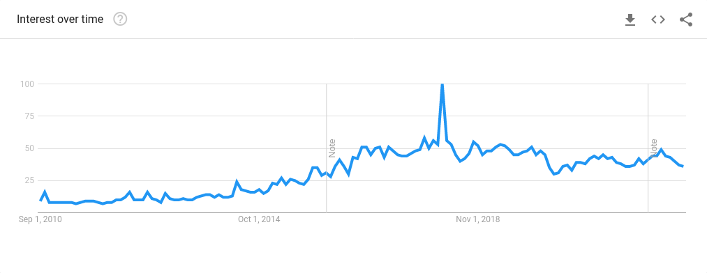
Self-driving cars

Google trends for 'Self-driving cars'

Lessons from aerospace

150 deaths per 10 billion miles

0.2 deaths per 10 billion miles

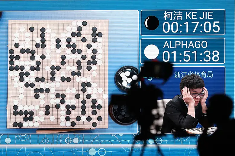
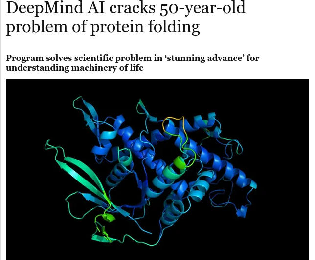
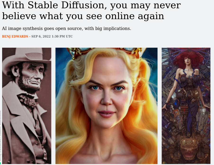
Artificial Intelligence

Why?

Bias-Variance trade-off

Image source: educative.io

Bayesian Learning

Image source: peterroelants.github.io Image source: educative.io

How to handle uncertainty safely?

My research area

My Background

- Navigation is the problem of converting sequence of observation to a sequence of actions for the purpose of going from one place to another. - It is often addressed in three parts. - Mapping---which is the estimation of the static part of the environment. - Localization---which is the estimation of the dynamic state of the environment like the agents location in the map. - and Planning which is the estimation of the sequence of action that moves the agent from current state to the desired goal. + Most of my work has been focused around mapping with some work around localization and planning. + Today I am going to talk about three of my works. + First I am going to talk about my work on making mapping faster by using modern inference methods on factor graphs. + Then I am going to talk about mutual localiztion that intern enables faster mapping by allowing robots to divide and conquer the environment. + In the end I will talk about making goal conditioned reinforcement learning faster by removing redundant computation.

Safety

Safe control while learning

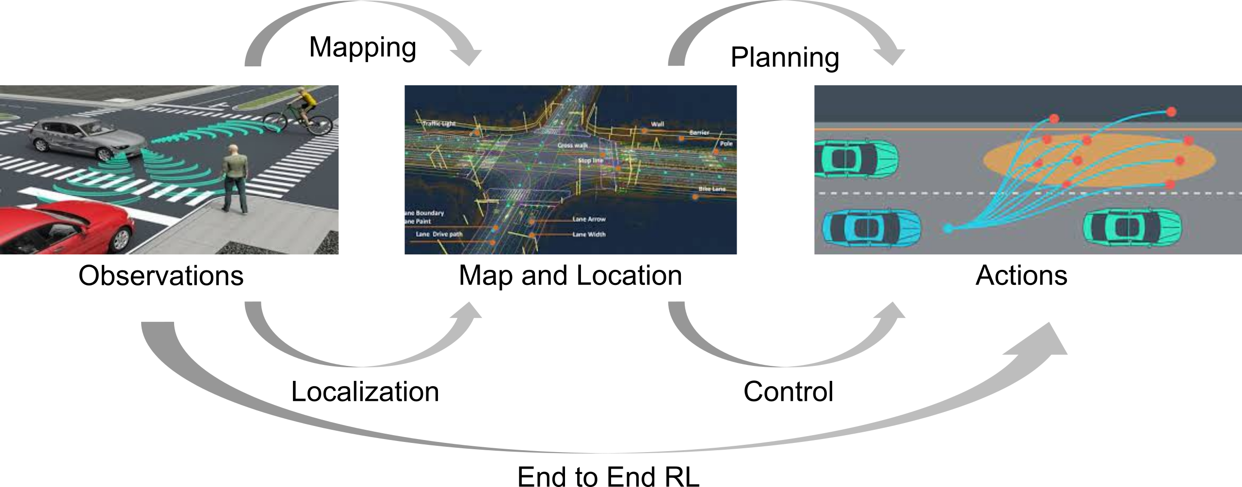
Given:

Map and localization
Desired trajectory as a plan
Unsafe regions

Problem 1:

Learn uncertainty aware robot system dynamics

Problem 2:

Follow trajectory avoiding unsafe actions

How to learn dynamics?

Maximum Likelihood models.
- Koopman operators ( Mamakoukas et al (2020) )
- Model based reinforcement Learning ( Wang et al (2019) )
Bayesian methods
- Ensemble neural networks ( Pearce et al (2018) )
- Dropout neural networks ( Gal and Ghahramani (2016) )
- Probabilistic Backpropagation ( Hernández-Lobato and Adams (2015) )
- Gaussian Processes (Rasmussen (2003))

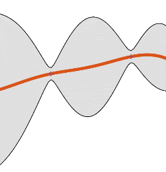
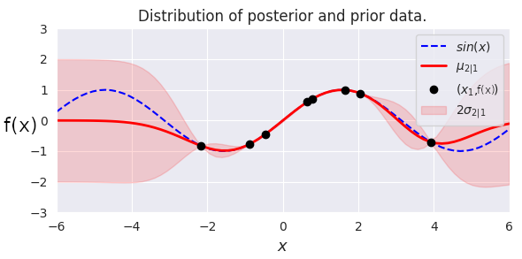
Gaussian Processes

Image source: https://peterroelants.github.io/

\[ \begin{bmatrix} f_1 \\ \vdots \\ f_n \end{bmatrix} \sim \calN\left( \begin{bmatrix} \mu_1 \\ \vdots \\ \mu_n \end{bmatrix}, \begin{bmatrix} \sigma_{1,1} & \dots & \sigma_{1,n} \\ \vdots & \dots & \vdots \\ \sigma_{n,1} & \dots & \sigma_{n,n} \end{bmatrix} \right) \]
\[ \begin{bmatrix} f(\bfx_1) \\ \vdots \\ f(\bfx_n) \end{bmatrix} \sim \calN\left( \begin{bmatrix} \mu(\bfx_1) \\ \vdots \\ \mu(\bfx_n) \end{bmatrix}, \begin{bmatrix} \sigma(\bfx_1,\bfx_1) & \dots & \sigma(\bfx_1,\bfx_n) \\ \vdots & \dots & \vdots \\ \sigma(\bfx_n,\bfx_1) & \dots & \sigma(\bfx_n, \bfx_n) \end{bmatrix} \right) \]
\[ f \sim \GP(\mu, \sigma) \]
\[ f(\bfx^*) | \{ f(\bfx_1) \dots f(\bfx_n) \} \sim \N( \mu_{*|n}(\bfx^*), \sigma_{*|n}(\bfx^*) ) \]

Problem formulation

\begin{align} \min_{\bfu \in \mathcal{U}}& \text{ Cost function } \\ \qquad\text{s.t.}&~~\bbP\bigl( \text{ Safety constraint } \bigr) \ge 1-\epsilon, \end{align}

Consider a robot tasked to cross a narrow bridge. In the scenario, the robot dynamics are not known with certainity, we want the robot to learn about its own dynamics to the point that it is safe to cross the bridge with a desired probability. Fragment 1: Specifically, we consider a control-affine system. And we write it in in a Linear-form using homogeneous coordinates. We denote homogeneous coordinates with an underline. Fragment 2: We assume that state-dependent part of the dynamics, capital F of x, is a Gaussian process whose mean and uncertainty could be estimated. Fragment 3: We want to formulate a controller that minimizes task cost function subject to the satisfaction of safety condition with a given probability $1-\epsilon $. A specific example of that would be to have an epsilon greedy unsafe controller. The safe controller will closely follow the unsafe controller constrained by safety. The epsilon greedy parts allows the robot to take random actions so that it can reduce the uncertainty of its dynamics.

Problem 1

\begin{align} \dot{\bfx} = F(\bfx) \ctrlaff \end{align}
\[ \vect(F(\bfx)) \sim \GP(\vect(\bfM_0(.)), \bfK_0(.,.)) \]
\[\StDat_{1:k} \triangleq [\bfx(t_1), \dots, \bfx(t_k)]\]
\[\bfU_{1:k} \triangleq [\bfu(t_1), \dots, \bfu(t_k)]\]
\[ \StDtDat_{1:k} \triangleq [\dot{\bfx}(t_1), \dots, \dot{\bfx}(t_k)] \]
Compute the posterior distribution $\calG\calP(\vect(\bfM_k(\bfx)), \bfK_k(\bfx,\bfx'))$ of $\vect(F(\bfx)) \mid (\StDat_{1:k}, \bfU_{1:k}, \StDtDat_{1:k})$.

Control Barrier Functions

For differentiable $ h(\bfx) $,
safe set is $ \calC = \{ \bfx \in \calX : h(\bfx) > 0 \} $
Assume $ \grad_\bfx h(\bfx) \ne 0 \quad \forall x \in \partial \calC $
Assume system starts in safe state $ \bfx(0) \in \calC $
System stays safe iff

\[ \dot{h}(\bfx) \ge - \gamma h(\bfx) \]
Ames et al (ECC 2019): \begin{multline} \text{ System stays safe } \Leftrightarrow~~\exists~\bfu = \pi(\bfx)~~\text{s.t.}\\ \mbox{CBC}(\bfx,\bfu) := [\grad_\bfx h(\bfx)]^\top F(\bfx)\ctrlaff + \gamma h(\bfx) \ge 0 \;~ \forall \bfx \in \calX. \end{multline}

Problem 2

\begin{align} \dot{\bfx} = F(\bfx) \ctrlaff \end{align}
\[ \vect(F(\bfx)) \sim \GP(\vect(\bfM_k(.)), \bfK_k(.,.)) \]
Find $\bfu_k$ and $\tau_k$ such that for $\bfu(t) = \bfu_k$ \[ \mathbb{P}(\mbox{CBC}(\bfx(t),\bfu_k) \ge 0) \ge p_k \] for all $ t \in [t_k,t_k+\tau_k) $

Approach

Estimate posterior distribution over $F(\bfx)$
Propagate uncertainty to the Safety condition.
Extension to continuous time using Lipschitz continuity assumptions.
Extension to higher relative degree systems.

\[ \vect(F(\bfx)) \sim \GP(\vect(\bfM_0(.)), \bfK_0(.,.)) \]

Decoupled GPs: Learn each element of $F(\bfx)$ independently: \[ \bfK_0(\bfx, \bfx') = \diag([\kappa(\bfx, \bfx'), \dots ]) \] No correlation across dimensions, training data still correlated.

Corregionalization models: Alvarez et al (FTML 2012): \[ \bfK_0(\bfx, \bfx') = \kappa(\bfx, \bfx') \boldsymbol{\Sigma} \] $\Sigma \in \R^{n(1+m) \times (1+m)n}$ has too many parameters to learn

Matrix Variate Gaussian: Inspired from Sun et al (AISTATS 2017)

\[ F \sim \mathcal{MVG}(\bfM, \bfA, \bfB) \Leftrightarrow \vect(F) \sim \calN(\vect(M), \bfB \otimes \bfA) \]

\[ \bfK_0(\bfx, \bfx') = \bfB_0(\bfx, \bfx') \otimes \bfA \]

Factorization assumption: \[ \vect(F(\bfx)) \sim \GP(\vect(\bfM_0(.)), \bfB_0(.,.) \otimes \bfA) \]

Directly learning the vectorized form of Gaussian Process in this form is hard to ensure positive definiteness of each output. That's why simplifying assumptions are used. For example, Alvarez et al reviewed a number of multi-output Gaussian processes that decompose the kernel into a scalar kernel that only depends on the input and an input independent matrix that captures the covariance between output components. However, this proposition is for vector-valued Gaussian processes and in our case the matrix Sigma will end up scaling poorly with the state dimension and control vector dimension. Another option from Sun et al considers a Matrix Variate Gaussian distribution, where the covariance between rows (B) and columns (A) is considered by separately. In vectorized form the covariance is just the kronecker product of row and column covariance matrices. This is the assumption that we use for Matrix Variate Gaussian process and factorize kernel K_0 into column covariance matrix A and row covariance matrix B. By assuming that only the row covariance matrix depends upon input, we will see that we get a nice structure in the inference result.

Matrix variate Gaussian Process

$ \newcommand{\prl}[1]{\left(#1\right)} \newcommand{\brl}[1]{\left[#1\right]} \newcommand{\crl}[1]{\left\{#1\right\}} $ \begin{equation} \begin{aligned} \vect(F(\bfx)) &\sim \mathcal{GP}(\vect(\bfM_0(\bfx)), \bfB_0(\bfx,\bfx') \otimes \bfA) %F(\bfx)\underline{\bfu} &\sim \mathcal{GP}(\bfM_0(\bfx)\underline{\bfu}, \underline{\bfu}^\top \bfB_0(\bfx,\bfx') \underline{\bfu}' \otimes \bfA) \end{aligned} \end{equation}

Given data $\StDat_{1:k}$, $\StDtDat_{1:k} $, and $ \underline{\boldsymbol{\mathcal{U}}}_{1:k} $.

\begin{equation*} \newcommand{\ubcalU}{\underline{\boldsymbol{\calU}}} \newcommand{\bcalM}{\boldsymbol{\calM}} \newcommand{\bcalB}{\boldsymbol{\calB}} \newcommand{\bcalC}{\boldsymbol{\calC}} \begin{aligned} &\bfM_k(\bfx) \triangleq \bfM_0(\bfx) + \left( \dot{\bfX}_{1:k} - \bcalM_{1:k}\ubcalU_{1:k}\right) \left(\ubcalU_{1:k}\bcalB_{1:k}(\bfx)\right)^\dagger \\ &\bfB_k(\bfx,\bfx') \triangleq \bfB_0(\bfx,\bfx') - \bcalB_{1:k}(\bfx)\ubcalU_{1:k} \left(\ubcalU_{1:k}\bcalB_{1:k}(\bfx')\right)^\dagger \\ &\left(\ubcalU_{1:k}\bcalB_{1:k}(\bfx)\right)^\dagger \triangleq \left(\ubcalU_{1:k}^\top\bcalB_{1:k}^{1:k}\ubcalU_{1:k} + \sigma^2 \bfI_k\right)^{-1}\ubcalU_{1:k}^\top\bcalB_{1:k}^\top(\bfx). \label{eq:mvg-posterior} \end{aligned} \end{equation*}

Inference on MVGP: \begin{align} \vect(F_k(\bfx_*)) &\sim \mathcal{GP}(\vect(\bfM_k(\bfx_*)), \; \bfB_k(\bfx_*,\bfx_*') \otimes \bfA). \\ F_k(\bfx_*)\underline{\bfu}_* &\sim \mathcal{GP}(\bfM_k(\bfx_*)\underline{\bfu}_*, \; \underline{\bfu}_*^\top\bfB_k(\bfx_*,\bfx_*')\underline{\bfu}_*\otimes\bfA). \end{align}

Next we describe how to do inference with the Matrix Variate Gaussian Process. Defining some notation regarding collected data. We collect trajectories with state, control and state derivative. If the state derivative is not available, we estimate it numerically. Note while most X data matrices are just row stacking of state vectors. The control data matrix is a diagonal matrix in homogeneous coordinates of control vector. Using some algebra using schur complement and typical Gaussian conditional distribution, we can compute mean matrix M_k and row covariance matrix B_k. Finally we get the inference result for Mean and variance of Matrix variate Gaussian process. Note that due to the choice of only row covariance matrix B depending upon input x, we get the same GP structure as we started with.

Learning Experiments

\begin{align} \begin{bmatrix} \dot{\theta} \\ \dot{\omega} \end{bmatrix} = \underbrace{\begin{bmatrix} \omega \\ -\frac{g}{l} \sin(\theta) \end{bmatrix}}_{f(\bfx)} + \underbrace{\begin{bmatrix} 0 \\ \frac{1}{ml} \end{bmatrix}}_{g(\bfx)} u \end{align}

Learning Experiments

Approach

Estimate $F(\bfx)$ with Matrix-Variate Gaussian Process
Propagate uncertainty to the Safety condition
Extension to continuous time using Lipschitz continuity assumptions.
Extension to higher relative degree systems.

Uncertainty propagation to CBC

\[ \mbox{CBC}(\bfx, \bfu)= \grad_\bfx h(\bfx)F_k(\bfx)\ctrlaff + \alpha(h(\bfx)) \]
Recall: \begin{equation} F_k(\bfx_*)\underline{\bfu}_* \sim \mathcal{GP}(\bfM_k(\bfx_*)\underline{\bfu}_*, \underline{\bfu}_*^\top\bfB_k(\bfx_*,\bfx_*')\underline{\bfu}_*\otimes\bfA). \end{equation}
Lemma : \[ \mbox{CBC}(\bfx, \bfu) \sim \GP(\E[\mbox{CBC}], \Var(\mbox{CBC})) \] \begin{align} \label{eq:parametofpi5543} \E[\mbox{CBC}_k](\bfx, \bfu) &= \nabla_\bfx h(\bfx)^\top \bfM_k(\bfx)\underline{\bfu} + \alpha(h(\bfx)),\\ \Var[\mbox{CBC}_k](\bfx, \bfx'; \bfu) &= \underline{\bfu}^\top\bfB_k(\bfx,\bfx')\underline{\bfu} \nabla_\bfx h(\bfx)^{\top}\bfA\nabla_\bfx h(\bfx') \end{align} Note: mean and variance are Affine and Quadratic in $ \bfu $ respectively.

Deterministic condition for controller

\begin{align} \min_{\bfu_k \in \mathcal{U}}& \text{ Cost function } \\ \qquad\text{s.t.}&~~\bbP\bigl( \text{ Safety constraint } \mid \bfx_k,\bfu_k \bigr) \ge 1-\epsilon, \end{align}

\begin{align} \min_{\bfu_k \in \mathcal{U}}& \text{ Quadratic cost function } \\ \qquad\text{s.t.}&~~\bbP\bigl( \style{color:red}{\mbox{CBC}(\bfx_k, \bfu_k) > \zeta > 0} \mid \bfx_k,\bfu_k \bigr) \ge 1-\epsilon, \end{align}
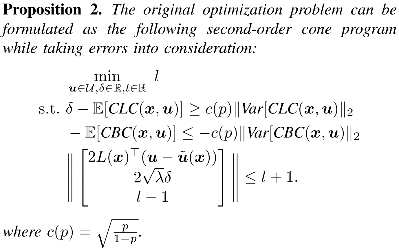
Safe controller (an SOCP): \begin{align} \min_{\bfu_k \in \mathcal{U}}& \text{ Quadratic cost function } \\ \qquad\text{s.t.}\qquad& \cssId{highlight-current-red-1}{\class{fragment}{ \E[\CBC] - \zeta \ge \sqrt{2\Var(\CBC)(\erf^{-1}(2\epsilon-1))^2} }} \end{align}

Recall the problem formulation. We want to ensure Safety constraint with some high probability. Fragment 1: More specifically, we want to ensure the Control Barrier Condition is greater than 0 by some margin zeta. Fragment 2: Since we have already shown that Control Barrier Condition is a Gaussian Process, we can analytically compute this probability in terms of mean and variance. Fragment 3: After some algebra we can convert the problem formulation into a nice Quadratically constrained Quadratic program with two conditions. Recall that the mean and variance of CBC are Affine and Quadratic in u respectively. Fragment 4: The first condition intuitively means that the CBC should be far from zeta by atleast by a term proportional to the standard deviation. The quadratic form of the first condition allows mean to be either side of zeta, but we want it to be greater than zeta which is greater than 0.

Approach

Estimate $F(\bfx)$ with Matrix-Variate Gaussian Process
Propagate uncertainty to the Control Barrier condition.
Extension to continuous time using Lipschitz continuity assumptions.
Extension to higher relative degree systems.

Safety beyond triggering times

So far: \begin{align} \min_{\bfu_k \in \mathcal{U}}& \|\bfR(\bfx) (\bfu_k - \pi_\epsilon(\bfx_k) \|_2^2 \\ \qquad\text{s.t.}&~~ \bbP\bigl( \mbox{CBC}(\style{color:red}{\bfx_k}, \bfu_k) > \style{color:red}{\zeta} \mid \bfx_k,\bfu_k \bigr) \ge \style{color:red}{1-\epsilon}, \end{align}
Next: \begin{align} \min_{\bfu_k \in \mathcal{U}}& \|\bfR(\bfx) (\bfu_k - \pi_\epsilon(\bfx_k) \|_2^2 \\ \qquad\text{s.t.}&~~ \bbP\bigl( \mbox{CBC}(\style{color:red}{\bfx(t)}, \bfu_k) > \style{color:red}{0} \mid \bfx_k,\bfu_k \bigr) \ge \style{color:red}{p_k}, \qquad \style{color:red}{\forall t \in [t_k, t_k + \tau_k)} \end{align}

Safety beyond triggering times

Assume Lipschitz continuity of dynamics: \begin{align} \textstyle \label{eq:smoth23} \bbP\left( \sup_{s \in [0, \tau_k)}\|F(\bfx(t_k+s))\ctrlaff_k -F(\bfx(t_k))\ctrlaff_k\| \le L_k \|\bfx(t_k+s)-\bfx_k\| \right) \ge q_k:=1-e^{-b_kL_k}. \end{align}
Assume Lipschitz continuity of $ \alpha(h(\bfx)) $: \begin{align} \label{htym6!7uytf} |\alpha \circ h(\bfx(t_k+s))-\alpha \circ h(\bfx_k)| \le L_{\alpha \circ h} \|\bfx(t_k+s)-\bfx_k\|. \end{align}
\[ \sup_{s \in [0, \tau_k)} \| \grad_\bfx h(x(t_k + s)) \| \le \chi_k \]

Theorem: \[ \bbP\bigl( \mbox{CBC}(\bfx_k, \bfu_k) > \zeta \mid \bfx_k,\bfu_k \bigr) \ge 1-\epsilon \quad\Rightarrow\quad \bbP\bigl( \mbox{CBC}(\bfx(t), \bfu_k) > 0 \mid \bfx_k,\bfu_k \bigr) \ge p_k, \; \forall t \in [t_k, t_k + \tau_k) \] holds with $ p_k = 1-\epsilon q_k $ and $ \tau_k \le \frac{1}{L_k}\ln\left(1+\frac{L_k\zeta}{(\chi_kL_k+L_{\alpha \circ h})\|\dot{\bfx}_k\|}\right) $

Approach

Estimate $F(\bfx)$ with Matrix-Variate Gaussian Process
Propagate uncertainty to the Control Barrier condition.
Extension to continuous time using Lipschitz continuity assumptions.
Extension to higher relative degree systems.

Higher relative degree CBFs

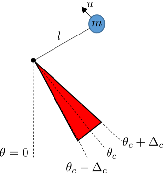
\begin{align} \begin{bmatrix} \dot{\theta} \\ \dot{\omega} \end{bmatrix} = \underbrace{\begin{bmatrix} \omega \\ -\frac{g}{l} \sin(\theta) \end{bmatrix}}_{f(\bfx)} + \underbrace{\begin{bmatrix} 0 \\ \frac{1}{ml} \end{bmatrix}}_{g(\bfx)} u \end{align}
\begin{align} h\left(\begin{bmatrix} \theta \\ \omega \end{bmatrix} \right) = \cos(\Delta_{col}) - \cos(\theta - \theta_c) \end{align}
Note that $ \underbrace{\grad_\bfx h(\bfx) g(\bfx)}_{\Lie_g h(\bfx)} = 0 $

$ \CBC(\bfx, \bfu) = \underbrace{[\grad_\bfx h(\bfx)]^\top f(\bfx)}_{\Lie_f h(\bfx)} + \underbrace{[\grad_\bfx h(\bfx)]^\top g(\bfx)}_{\Lie_g h(\bfx)} \bfu + \alpha(h(\bfx)) $
is independent of $\bfu$.

Exponential Control Barrier Functions (ECBF)

\[ \CBCr(\bfx, \bfu) := \Lie_f^{(r)} h(\bfx) + \cssId{highlight-current-red-1}{\class{fragment}{ \underbrace{ \Lie_g \Lie_f^{(r-1)} h(\bfx) }_{\ne 0} }} \bfu + \bfk_\alpha^\top \begin{bmatrix} h(\bfx) \\ \Lie_f h(\bfx) \\ \vdots \\ \Lie_f^{(r-1)} h(\bfx) \end{bmatrix} \]

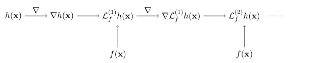
Propagating uncertainty to $ \CBCtwo $

\[ \CBCtwo(\bfx, \bfu) = [\grad_\bfx \Lie_f h(\bfx)]^\top F(\bfx)\ctrlaff + \bfk_\alpha^\top \begin{bmatrix} h(\bfx) & \Lie_f h(\bfx) \end{bmatrix}^\top \]
$ \Lie_f h(\bfx) = \grad_x h(\bfx) f(\bfx) $ is a Gaussian process
$ \grad_\bfx \Lie_f h(\bfx) $ is a Gaussian process
- If $ p(\bfx) \sim \GP(\mu(\bfx), \kappa(\bfx, \bfx'))$, then
  $ \grad_\bfx p(\bfx) \sim \GP(\grad_\bfx \mu(\bfx), H_\bfx \kappa(\bfx, \bfx')) $

Propagating uncertainty to $ \CBCtwo $

\[ \CBCtwo(\bfx, \bfu) = [\grad_\bfx \Lie_f h(\bfx)]^\top F(\bfx)\ctrlaff + \bfk_\alpha^\top \begin{bmatrix} h(\bfx) & \Lie_f h(\bfx) \end{bmatrix}^\top \]
$ \Lie_f h(\bfx) = \grad_x h(\bfx) f(\bfx) $ is a Gaussian process
$ \grad_\bfx \Lie_f h(\bfx) $ is a Gaussian process
$ [\grad_\bfx \Lie_f h(\bfx)]^\top F(\bfx)\ctrlaff $ is a quadratic form of GP (not a GP )
$ \CBCtwo(\bfx, \bfu) $ is a quadratic form of GP.
$ \E[\CBCtwo](\bfx, \bfu) $ is still affine in $ \bfu $.
$ \Var[\CBCtwo](\bfx, \bfx'; \bfu) $ is still quadratic in $ \bfu $.

Now that we have defined CBCtwo as the safety condition, we want to see a how to propagate uncertainty to CBCtwo. We have already seen that Lie derivative of h wrt to f is a gaussian process. The gradients of GPs are GPs, hence the gradient of Lie of h of x is also a GP. The dot product of this gradient with system dynamics is a quadratic form of two GPs. Now this is not a GP. But its mean and variacne can be computed analyticallly. Note that CBCtwo is affine in this term which is again a quadratic form in GP. Without writing the long expressions for the mean and variance of CBCtwo, I want to convey to you two things; that mean and variance of CBCtwo can be computed analytically and the mean and variance of CBCtwo are affine and quadratic in control signal like CBCone.

Extending to $\CBCr$

\[ \CBCr(\bfx, \bfu) = [\grad_\bfx \Lie_f^{(r)} h(\bfx)]^\top F(\bfx)\ctrlaff + \bfk_\alpha^\top \begin{bmatrix} h(\bfx) & \Lie_f h(\bfx) & \dots \Lie_f^{(r-1)} h(\bfx) \end{bmatrix}^\top \]
$ \CBCr(\bfx, \bfu) $ is not a GP
$ \E[\CBCr](\bfx, \bfu) $ is still affine in $ \bfu $.
$ \Var[\CBCr](\bfx, \bfx'; \bfu) $ is still quadratic in $ \bfu $.
For $ r \ge 3 $, $\CBCr$ statistics can be estimated by Monte-carlo methods.

Safe controller using ECBF

\begin{align} \min_{\bfu_k \in \mathcal{U}}& \|\bfR(\bfx) (\bfu_k - \pi_\epsilon(\bfx_k) \|_2^2 \\ \qquad\text{s.t.}&~~ \bbP\bigl( \CBCr(\bfx_k, \bfu_k) > \zeta \mid \bfx_k,\bfu_k \bigr) \ge 1-\epsilon \end{align}
Using Cantelli's (Chebyshev's one-sided) inequality
Safe controller (an SOCP) \begin{align} \min_{\bfu_k \in \mathcal{U}}& \|\bfR(\bfx) (\bfu_k - \pi_\epsilon(\bfx_k) \|_2^2 \\ \qquad\text{s.t.}\qquad &\E[\mbox{CBC}_k^{(r)}]-\zeta \ge \sqrt{\frac{1-\epsilon}{\epsilon}\Var[\mbox{CBC}_k^{(r)}]} \end{align}

Safe controller using ECBF Experiments

\begin{align} \begin{bmatrix} \dot{\theta} \\ \dot{\omega} \end{bmatrix} = \underbrace{\begin{bmatrix} \omega \\ -\frac{g}{l} \sin(\theta) \end{bmatrix}}_{f(\bfx)} + \underbrace{\begin{bmatrix} 0 \\ \frac{1}{ml} \end{bmatrix}}_{g(\bfx)} u \end{align}
\begin{align} h\left(\begin{bmatrix} \theta \\ \omega \end{bmatrix} \right) = \cos(\Delta_{col}) - \cos(\theta - \theta_c) \end{align}

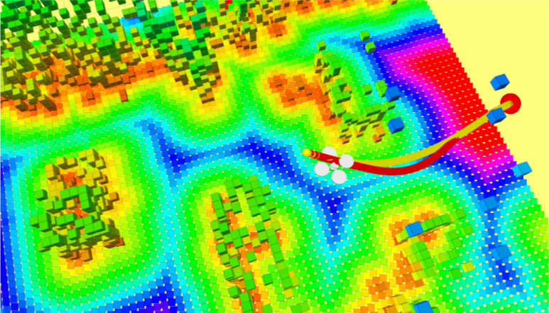
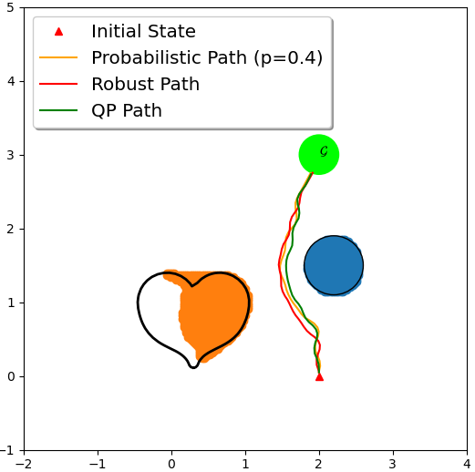
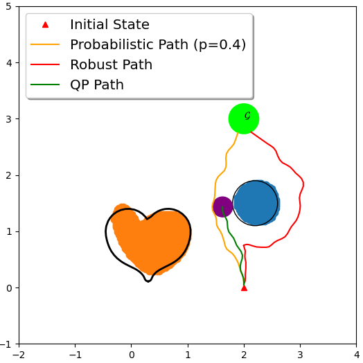
Ackerman Drive Simulations

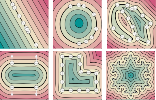
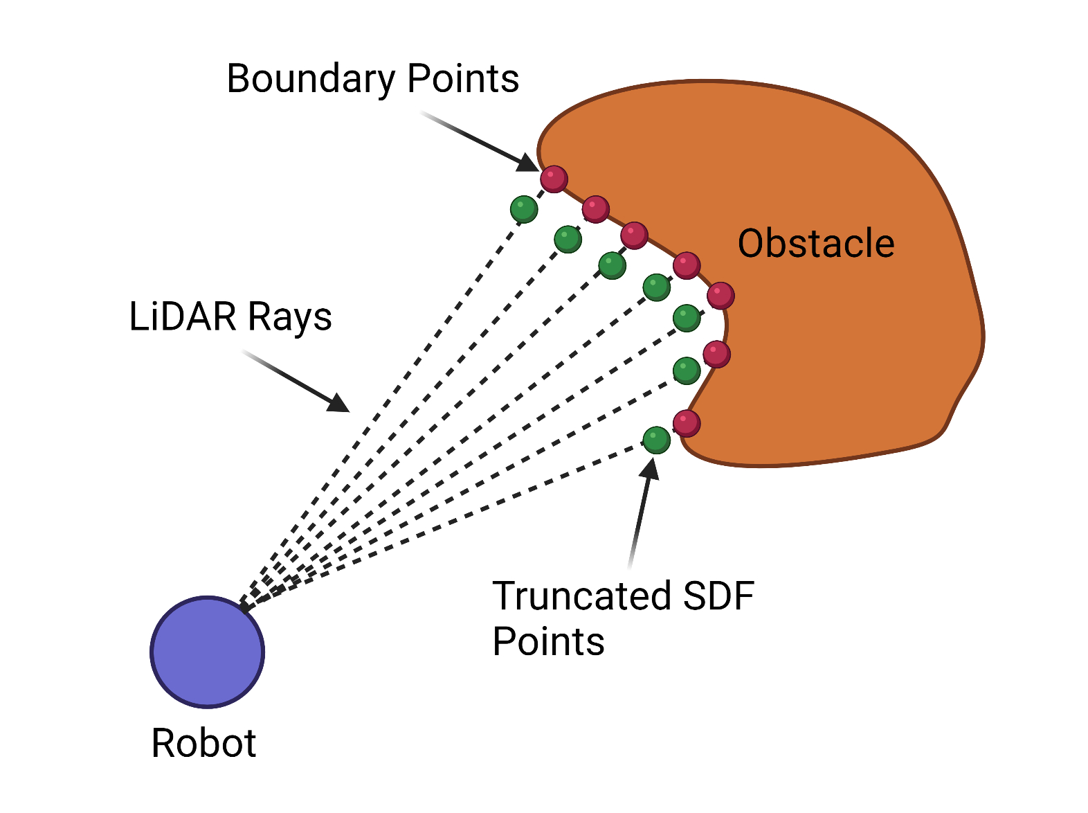
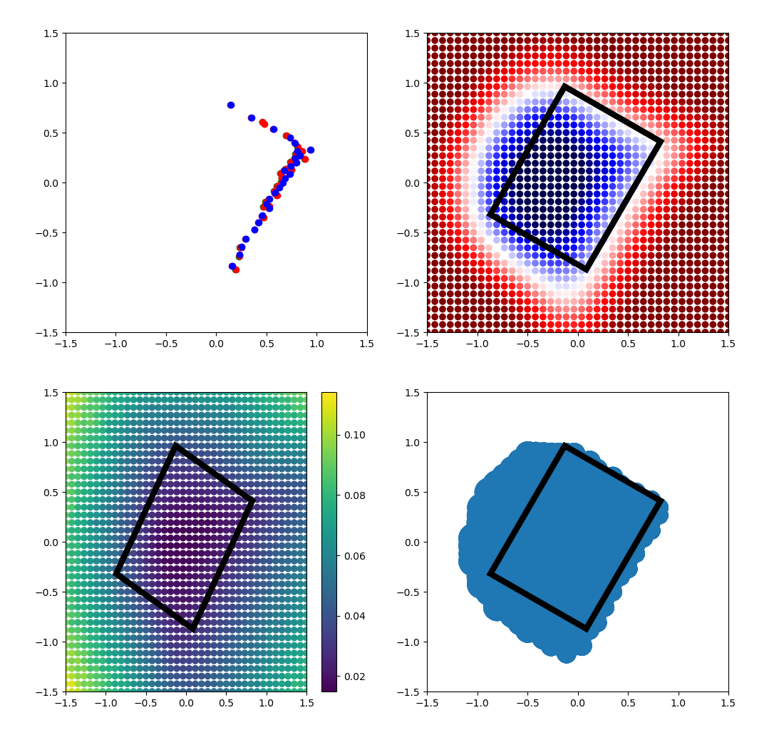
2022 upgrade: Learning $ h(\bfx) $

“Fiesta” Han et al (IROS 2019), Gropp et al (ICML 2020)

Better math

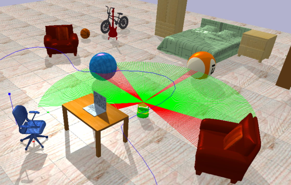
Better Simulation: PyBullet

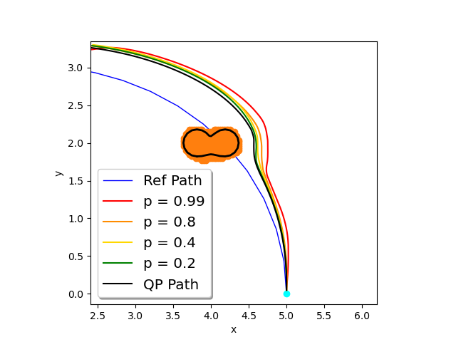
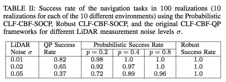
Results

Sample trajectories

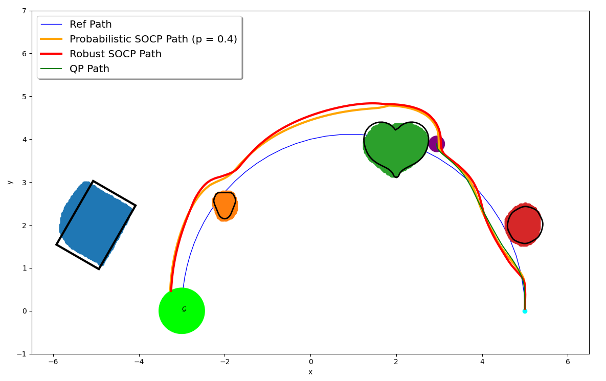
Take away

Bayesian learning enables uncertainty-awareness
Uncertainty-aware controller can be formulated as SOCP controller

Future work

Other work

OrcVIO

Mutual Localization

Learning from Interventions

Continuous occlusion modeling

Visual Inertial Odometry

Mutual Localization

Learning from Interventions

Continuous occlusion modeling

Other work

OrcVIO

Mutual Localization

Semantic Inverse RL

Learning from Interventions

Future work

Collaborators

Questions?

OrcVIO

Mutual Localization

vikasdhiman.info

Inverse Reinforcement Learning

Learning from Interventions

Shengyang Sun, Changyou Chen, and Lawrence Carin. Learning Structured Weight Uncertainty in Bayesian Neural Networks. In International Conference on Artificial Intelligence and Statistics (AISTATS), pages 1283–1292, 2017.
A. D. Ames, S. Coogan, M. Egerstedt, G. Notomista, K. Sreenath, and P. Tabuada. Control barrier functions: Theory and applications. In 2019 18th European Control Conference (ECC), pages 3420–3431, June 2019. doi: 10.23919/ECC.2019.8796030.
Mauricio A Alvarez, Lorenzo Rosasco, and Neil D Lawrence. Kernels for vector-valued functions: A review. Foundations and Trends in Machine Learning, 4(3):195–266, 2012.
Niranjan Srinivas, Andreas Krause, Sham M Kakade, and Matthias Seeger. Gaussian process opti- mization in the bandit setting: No regret and experimental design. arXiv preprint arXiv:0912.3995, 2009.
Quan Nguyen and Koushil Sreenath. Exponential control barrier functions for enforcing high relative- degree safety-critical constraints. In 2016 American Control Conference (ACC), pages 322–328. IEEE, 2016a.
Louizos, Christos, and Max Welling. "Structured and efficient variational deep learning with matrix gaussian posteriors." International Conference on Machine Learning. 2016.
Khojasteh, M. J., Dhiman, V., Franceschetti, M., & Atanasov, N. (2020). Probabilistic safety constraints for learned high relative degree system dynamics. L4DC 2020. available https://arXiv.org/abs/1912.10116.
Learning from Interventions using Hierarchical Policies for Safe Learning J Bi, V Dhiman, T Xiao, C Xu - AAAI 2020. Available https://arXiv.org/abs/1912.02241
Learning Navigation Costs from Demonstration in Partially Observable Environments T Wang, V Dhiman, N Atanasov. ICRA 2020. Available https://arXiv.org/abs/2002.11637
Andrychowicz, Marcin, et al. "Hindsight experience replay." Advances in Neural Information Processing Systems. 2017.
Mutual localization: Two camera relative 6-dof pose estimation from reciprocal fiducial observation. V Dhiman, J Ryde, JJ Corso. IROS 2013
Learning Compositional Sparse Models of Bimodal Percepts. S Kumar, V Dhiman, JJ Corso AAAI, 2014
Voxel planes: Rapid visualization and meshification of point cloud ensembles. J Ryde, V Dhiman, R Platt IROS, 2013
Modern MAP inference methods for accurate and fast occupancy grid mapping on higher order factor graphs. V Dhiman, A Kundu, F Dellaert, JJ Corso ICRA 2014
Continuous occlusion models for road scene understanding M Chandraker, V Dhiman. US Patent 9,821,813, 2017
A continuous occlusion model for road scene understanding V Dhiman, QH Tran, JJ Corso, M Chandraker. CVPR 2016
A Critical Investigation of DRL for Navigation V Dhiman, S Banerjee, B Griffin, JM Siskind, JJ Corso NeurIPS DRL Workshop, 2017.
Learning Compositional Sparse Bimodal Models S Kumar, V Dhiman, PA Koch, JJ Corso. PAMI, 2017.
(Mirowski et al. 2017) Learning to navigate in complex environments. In ICLR 2017.
Multi-Goal Reinforcement Learning: Challenging Robotics Environments and Request for Research. Matthias Plappert and Marcin Andrychowicz and Alex Ray and Bob McGrew and Bowen Baker and Glenn Powell and Jonas Schneider and Josh Tobin and Maciek Chociej and Peter Welinder and Vikash Kumar and Wojciech Zaremba. ArXiV 2018. 1802.09464
Kaelbling, Leslie Pack. "Learning to achieve goals." IJCAI. 1993.
V. Dhiman, S. Banerjee, J. M. Siskind, and J. J. Corso. Learning goal-conditioned value functions with one-step path rewards rather than goal-rewards. In Submitted to ICLR, 2019. Under review.
Zachariou, Peter et al. “SPEEDING Effects on hazard perception and reaction time.” (2011).
Mnih, Volodymyr, et al. "Human-level control through deep reinforcement learning." Nature 518.7540 (2015): 529.
Watkins, Christopher JCH, and Peter Dayan. "Q-learning." Machine learning 8.3-4 (1992): 279-292.
Pearl, Judea. "Fusion, propagation, and structuring in belief networks." Artificial intelligence 29.3 (1986): 241-288.
Jojic, Vladimir, Stephen Gould, and Daphne Koller. "Accelerated dual decomposition for MAP inference." ICML. 2010.
Merali, Rehman S., and Timothy D. Barfoot. "Occupancy grid mapping with Markov chain monte carlo Gibbs sampling." Robotics and Automation (ICRA), 2013 IEEE International Conference on. IEEE, 2013.
Shayle R Searle and Marvin HJ Gruber.Linear models. John Wiley & Sons, 1971
Kehan Long, Vikas Dhiman, Melvin Leok, Jorge Cortés, Nikolay Atanasov: Safe Control Synthesis With Uncertain Dynamics and Constraints. IEEE Robotics Autom. Lett. 7(3): 7295-7302 (2022)