Continuous Optimization - Neural Networks

Reading: Chapter 7: MML Book

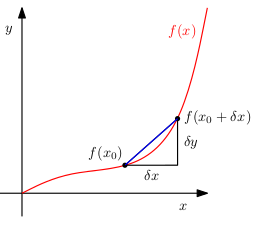
Recall geometry of a derivative¶

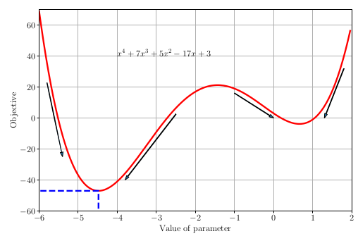
Minimizing general functions¶

We cannot minimize general functions by solving

\frac{\p f(\bfx)}{\p \bfx} = \mathbf{0}^\top

(1)

because the equation might not have a formula for it.

Instead we use iterative methods like gradient descent minimize general function $f(\bfx)$ .

Definition (Directional derivative)¶

Directional dervivative of a function $f(\bfx) : \bbR^n \to \bbR$ with respect to a given unit vector $\hat{\bfu} \in \bbR^n | \|\hat{\bfu}\| = 1$ is defined as

D_\bfu f(\bfx) = \lim_{\epsilon \to 0} \frac{f(\bfx + \epsilon \hat{\bfu}) - f(\bfx)}{\epsilon}

(2)

Ref Khan Academy

Ref Libretexts

Vector calculus chain rule (a theorem)¶

Given a function composition $\bff(\bfx) = \bfg(\bfh(\bfx)) = (\bfg \circ \bfh)(\bfx)$ where $\bfh : \bbR^n \to \bbR^m$ , $\bfg : \bbR^m \to \bbR^p$ and $\bfh: \bbR^m \to \bbR^p$

\frac{\p \bff}{\p \bfx} = \frac{\p \bff}{\p \bfh}\frac{\p \bfh}{\p \bfx}

(3)

or denoting the derivatives as Jacobian matrices we have,

\calJ_\bfx \bff = \calJ_\bfh[\bff] \calJ_\bfx [ \bfh ]

(4)

Theorem (Directional derivative is gradient dot product with the direction)¶

Express the trajectory in the direction $\bfu$ as a function of time $t$ as

\bfg(t) = \bfx + t \hat{\bfu}

(5)

Note that the Jacobian of $\bfg(t)$ wrt $t$ is simply $\bfu$ ,

\calJ_t \bfg(t) = \hat{\bfu}

(6)

Recall the definition of directional derivative,

D_\bfu f(\bfx) = \lim_{\epsilon \to 0} \frac{f(\bfx + \epsilon \hat{\bfu}) - f(\bfx)}{\epsilon}.

(7)

Compare it with the derivative of $f(\bfg(t))$ with respect to $t$ at $t=0$

\frac{\p f(\bfg(t))}{\p t} = \lim_{\epsilon \to 0} \frac{f(\bfx + (t + \epsilon) \hat{\bfu}) - f(\bfx + t\hat{\bfu})}{\epsilon} \Big\vert_{t = 0}.

(8)

\frac{\p f(\bfg(t))}{\p t} = \lim_{\epsilon \to 0} \frac{f(\bfx + \epsilon \hat{\bfu}) - f(\bfx )}{\epsilon} = D_\bfu f(\bfx).

(9)

We can compute $\frac{\p f(\bfg(t))}{\p t}$ by chain rule,

D_\bfu f(\bfx) = \calJ_t f(\bfg(t)) = \calJ_\bfx f(\bfx) \calJ_t \bfg = \nabla_\bfx^\top f(\bfx) \hat{\bfu}

(10)

Theorem : The direction of stepest ascent and descent¶

Let $\hat{\bfu}$ be of unit magnitude. The directional derivative represents how the function changes in the direction $\hat{\bfu}$ .

D_{\hat{\bfu}} f(\bfx) = \nabla_\bfx^\top f(\bfx) \hat{\bfu} = \|\nabla_\bfx f(\bfx)\|\cos(\theta),

(11)

where $\theta$ is the angle between $\nabla_\bfx f(\bfx)$ and $\hat{\bfu}$ . The change is maximum when $\theta = 0$ and $\cos(\theta) = 1$ and the change is minimum when $\theta = 180^\circ$ and $\cos(\theta) = -1$ .

In other words the function $f$ increases the most (stepest ascent) when $\hat{\bfu} \propto \nabla_\bfx f(\bfx)$ and decreases the most (steepest descent) when $\hat{\bfu} \propto - \nabla_\bfx f(\bfx)$ .

Gradient descent method¶

(Section 9.3 of Convex Optimization by Stephen Boyd and Lieven Vandenberghe)

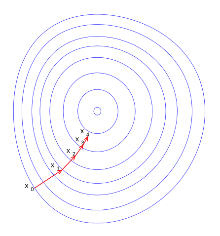
Start from a random point $\bfx_0$ , $\bfx_t \leftarrow \bfx_0$ .
Move in the direction opposite to $\nabla_\bfx f(\bfx)$ . If we were at $\bfx_t$ , then the next point is at $\bfx_{t+1} = \bfx_t - \alpha_t \nabla_\bfx f(\bfx)$ , where $\alpha_t > 0$ is a positive scalar, called the step size or the learning rate.
Stop when the gradient is almost zero $\|\nabla_\bfx f(\bfx)\| < 10^{-4}$ .

This corresponds to the following algorithm:

$\bfx_t = \bfx_0$
while ( $\|\nabla_\bfx f(\bfx)\| > 10^{-4}$ ) { $\bfx_t \leftarrow \bfx_t - \alpha_t \nabla_\bfx f(\bfx)$ }

Algorithm 9.3 Gradient descent method.

given a starting point $\bfx \in \text{dom}{f}$ .

repeat

$\Delta x = -\nabla f(\bfx)$ .
Choose step size $\alpha$
Update. $\bfx := \bfx + \alpha \bfx$

until stopping criterion is satisfied.

Gradient visualization¶

import matplotlib.pyplot as plt
import numpy as np
from matplotlib import animation, rc
rc('animation', html='jshtml')
def plot_gradients(func, gradfunc):
    x, y = np.mgrid[-3:3:21j,
                    -3:3:21j]
    bfx = np.array([x, y])
    f = func(x,y)
    [dfdx, dfdy] = gradfunc(x,y)
    fig, ax = plt.subplots()
    ctr = ax.contour(x, y, f, 20, cmap='Blues_r')
    ax.quiver(x, y, dfdx, dfdy)
    ax.plot([0], [0], 'ro') 
    ax.text(0, 0, '$x^*$', color='r')
    ax.set_xlabel('$x$')
    ax.set_ylabel('$y$')
    plt.show()

def f(x, y): return  x**2 + y**2
def gradf(x, y): return 2*x, 2*y
plot_gradients(f, gradf)

Quadratic function example:¶

A quadratic function $f(\bfx) = x_1^2 + x_2^2$ has level sets as circles:

S(f, c) = \{\bfx : x_1^2 + x_2^2 = c\}

(12)

It has the parameteric form as

S(f, c) = \{\bfg(c, \theta) = \begin{bmatrix}\sqrt{c} \cos(\theta) \\ \sqrt{c} \sin(\theta)\end{bmatrix} : \theta \in [0, 2\pi)\}

(13)

The gradient is:

\nabla_\bfx f(\bfx)^\top = 2\bfx^\top = 2 \begin{bmatrix} \sqrt{c} \cos(\theta) & \sqrt{c} \sin(\theta)\end{bmatrix}

(14)

and

The derivative of curve with respect to $\theta$ the tangent to the curve:

\calJ_\theta \bfg(c, \theta) = \begin{bmatrix} \frac{\p }{\p \theta} \sqrt{c} \cos(\theta) \\ \frac{\p }{\p \theta} \sqrt{c} \sin(\theta)\end{bmatrix} = \begin{bmatrix}-\sqrt{c} \sin(\theta) \\ \sqrt{c} \cos(\theta)\end{bmatrix}

(15)

\nabla_\bfx f(\bfx)^\top\calJ_\theta \bfg(c, \theta) = 2 \begin{bmatrix} \sqrt{c} \cos(\theta) & \sqrt{c} \sin(\theta)\end{bmatrix} \begin{bmatrix}-\sqrt{c} \sin(\theta) \\ \sqrt{c} \cos(\theta)\end{bmatrix} = 0

(16)

Taylor series approximation¶

A bit more about the step size/learning rate¶

Taylor series expansion originates from integration by parts

The fundamental theorem of calculus states that

f(x)=f(a)+\int _{a}^{x}\,f'(t)\,dt

(17)

Now we can integrate by parts and use the fundamental theorem of calculus again to see that

\begin{align} f(x)&=f(a)+{\Big (}xf'(x)-af'(a){\Big )}-\int _{a}^{x}tf''(t)\,dt\\&=f(a)+x\left(f'(a)+\int _{a}^{x}f''(t)\,dt\right)-af'(a)-\int _{a}^{x}tf''(t)\,dt\\&=f(a)+(x-a)f'(a)+\int _{a}^{x}\,(x-t)f''(t)\,dt, \end{align}

(18)

Recall the Taylor series expansion of a function $f(x)$ around $x_0$

f(x) = f(x_0) + \frac{d f(x)}{d x} (x - x_0) + \frac{1}{2!} \frac{d^2 f(x)}{d x^2} (x - x_0)^2 + \dots + \frac{1}{n!} \frac{d^n f(x)}{d x^n} (x - x_0)^n + \dots

(19)

Vectorized Taylor series expansion is

f(\bfx) = f(\bfx_0) + \nabla_\bfx^\top f(\bfx) (\bfx - \bfx_0) + \frac{1}{2!} (\bfx - \bfx_0)^\top \calH f(\bfx) (\bfx - \bfx_0)^\top + \dots \infty

(20)

While optimizing around the point $\bfx_t$ , we can use the Taylor series expansion to find a local quadratic approximation to find the next best minima:

\hat{f}(\bfx_{t+1}) = f(\bfx_t) + \nabla_\bfx^\top f(\bfx) (\bfx_{t+1} - \bfx_t) + \frac{1}{2!} (\bfx_{t+1} - \bfx_t)^\top \calH f(\bfx) (\bfx_{t+1} - \bfx_t)^\top

(21)

At the optimal point of the quadratic approximation the derivative is zero:

\frac{\p \hat{f}(\bfx_{t+1})}{\p \bfx_{t+1}} = \mathbf{0}^\top

(22)

\nabla_\bfx^\top f(\bfx) + (\bfx_{t+1} - \bfx_t)^\top \calH f(\bfx) = \mathbf{0}^\top

(23)

Taking transpose and rearranging the terms we get:

\bfx_{t+1} - \bfx_t = -[\calH f(\bfx)]^{-1}\nabla_\bfx f(\bfx)

(24)

\bfx_{t+1} = \bfx_t -[\calH f(\bfx)]^{-1}\nabla_\bfx f(\bfx)

(25)

This is the update rule for the Newton’s method for optimization. Note that the step size here is inversely proportional the second derivative.

Taylor series approximation¶

Approximate the following function to a quadratic function near the point $\bfx_0 = [-2, 3]$

$f (x) = 0.06\exp( 2x_1 +x_2) + 0.05\exp(x_1−2 x_2) + \exp(−x_1)$

f(\bfx) = 0.06 \exp([2, 1]\bfx) + 0.05 \exp([1, -2]\bfx) + \exp([-1, 0]\bfx)

(26)

Let $\bfb_1^\top = [2, 1]$ , $\bfb_2^\top = [1, -2]$ , $\bfb_3^\top = [-1, 0]$ .

\nabla_\bfx^\top f(\bfx) = 0.06 \bfb_1^\top \exp(\bfb_1^\top\bfx) + 0.05 \bfb_2^\top\exp(\bfb_2^\top\bfx) + \bfb_3^\top\exp(\bfb_3^\top\bfx)

(27)

\nabla_\bfx f(\bfx) = 0.06 \bfb_1 \exp(\bfb_1^\top\bfx) + 0.05 \bfb_2 \exp(\bfb_2^\top\bfx) + \bfb_3\exp(\bfb_3^\top\bfx)

(28)

H f(\bfx) = \nabla_\bfx^\top (\nabla_\bfx f(\bfx)) = 0.06 \bfb_1 \exp(\bfb_1^\top\bfx) \bfb_1^\top + 0.05 \bfb_2 \exp(\bfb_2^\top\bfx) \bfb_2^\top + \bfb_3\exp(\bfb_3^\top\bfx)\bfb_3^\top

(29)

H f(\bfx) = 0.06 \exp(\bfb_1^\top\bfx) \bfb_1 \bfb_1^\top + 0.05 \exp(\bfb_2^\top\bfx) \bfb_2 \bfb_2^\top + \exp(\bfb_3^\top\bfx)\bfb_3\bfb_3^\top

(30)

# Define the function
def f(x):
    
    """
    1. For an input x of shape x.shape = (2,) 
        f(x) must return a scalar
        
    2. For an input x of shape x.shape = (m, 2), 
        f(x) must return an array of shape (m,) 
        which contains f(x) is computed for m values of x

    3. For an input x of shape x.shape = (m, n, 2)
        f(x) must return an array of shape (m, n) 
        which contains f(x) is computed for (m x n) values of x
    """
    return (0.06 * np.exp(x @ [2, 1]) 
            + 0.05* np.exp(x @ [1, -2]) 
            + np.exp(x @ [-1, 0]))

# Compute its derivative, the gradient function
def grad_f(x):     
    """
    1. For an input x of shape x.shape = (2,) 
        grad_f(x) must return a n array of shape (2,)
        
    2. For an input x of shape x.shape = (m, 2), 
        grad_f(x) must return an array of shape (m, 2) 
        which contains grad_f(x) is computed for m values of x

    3. For an input x of shape x.shape = (m, n, 2)
        grad_f(x) must return an array of shape (m, n, 2) 
        which contains grad_f(x) is computed for (m x n) values of x
    """
    coeff1 = np.array([2, 1])
    coeff2 = np.array([1, -2])
    coeff3 = np.array([-1, 0])
    # Slicing using np.newaxis or None, increases the dimension by 1.
    # https://numpy.org/doc/stable/reference/constants.html#numpy.newaxis
    return (0.06 * np.exp(x @ coeff1)[..., None] * coeff1
            + 0.05 * np.exp(x @ coeff2)[..., None] * coeff2
            + np.exp(x @ coeff3)[..., None] * coeff3)

def numerical_jacobian(f, x, h=1e-10):
    n = x.shape[-1]
    eye = np.eye(n)
    x_plus_dx = x + h * eye # n x n
    num_jac = (f(x_plus_dx) - f(x)) / h # limit definition of the formula # n x m
    if num_jac.ndim >= 2:
        num_jac = num_jac.swapaxes(-1, -2) # m x n
    return num_jac
    
# Compare our grad_f with numerical gradient
def check_numerical_jacobian(f, jac_f,  nD=2, **kwargs):
    x = np.random.rand(nD)
    num_jac = numerical_jacobian(f, x, **kwargs)
    return np.allclose(num_jac, jac_f(x), atol=1e-06, rtol=1e-4) # m x n

## Throw error if grad_f is wrong
assert check_numerical_jacobian(f, grad_f)

## Gradient of gradient
def hessian_f(x):
    """
    1. For an input x of shape x.shape = (2,) 
        hessian_f(x) must return a n array of shape (2, 2)
        
    2. For an input x of shape x.shape = (m, 2), 
        hessian_f(x) must return an array of shape (m, 2, 2) 
        which contains hessian_f(x) is computed for m values of x

    3. For an input x of shape x.shape = (m, n, 2)
        hessian_f(x) must return an array of shape (m, n, 2, 2) 
        which contains hessian_f(x) is computed for (m x n) values of x 
    """
    coeff1 = np.array([2, 1])
    coeff2 = np.array([1, -2])
    coeff3 = np.array([-1, 0])
    return (0.06 * np.exp(x @ coeff1)[..., None, None] * np.outer(coeff1, coeff1)
            + 0.05 * np.exp(x @ coeff2)[..., None, None] * np.outer(coeff2, coeff2)
            +  np.exp(x @ coeff3)[..., None, None] * np.outer(coeff3, coeff3))

## Throw error if hessian_f is wrong
assert check_numerical_jacobian(grad_f, hessian_f)


def taylor_series_quad_approx(x0, func, grad_func, hessian_func):
    def quad_func(x):
        x_min_x0 = (x-x0)[..., None] # make column vectors
        x_min_x0_T = (x-x0)[..., None, :] # make row vectors
        grad_f_x0_T = grad_func(x0)[..., None, :] # make row vectors
        return (func(x0) 
                + grad_f_x0_T @ x_min_x0
                + x_min_x0_T @ hessian_func(x0) @ x_min_x0).squeeze(axis=(-1,-2))
            
    return quad_func

def plot_contours(func, ax=None, cmap='Blues_r', levels=20, 
                  xrange=slice(-3,3,21j),
                  yrange=slice(-3,3,21j)):
    x, y = np.mgrid[xrange,
                    yrange]
    bfx = np.concatenate([x[..., None],
                          y[..., None]], axis=-1)
    f = func(bfx)
    if ax is None:
        fig, ax = plt.subplots()
    ctr = ax.contour(x, y, np.log(f), levels, cmap=cmap)
    ax.clabel(ctr, ctr.levels, inline=True, fontsize=6)
    ax.set_xlabel('$x$')
    ax.set_ylabel('$y$')
    return ax
    
# Fit a quadratic curve around this curve:
ax = plot_contours(f, 
                   levels=[0.01, 0.5, 0.8, 1.0, 1.2, 1.6, 1.8, 2.0])
x0 = np.array([0, 2])
ax.plot([x0[0]], [x0[1]], 'ro')
ax.text(x0[0], x0[1], '$x_0$')
quad_func = taylor_series_quad_approx(x0, f, grad_f, hessian_f)
# x, y = np.mgrid[-3:3:21j,
#                     -3:3:21j]
# bfx = np.concatenate([x[..., None],
#                       y[..., None]], axis=-1)
# print(bfx.shape)
# print(f(bfx).shape)
# print(grad_f(bfx).shape)
# print(quad_func(bfx).shape)
plot_contours(quad_func, ax=ax, cmap='Reds_r', 
              levels=[0.1, 0.2, 0.5, 0.8, 1.0, 1.5],
              xrange=slice(-1,2,21j),
              yrange=slice(-2,3,21j))
ax.set_title("Taylor series quadratic fit in red to the blue curve")
plt.show()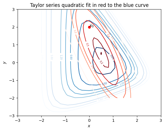

Example Taylor series 1¶

Following the example above, fit a quadratic function to the function using Taylor series expansion near the points $\bfx_0 = \begin{bmatrix} -1 \\ 1\end{bmatrix}$ then visualize the contour plots of the original function and the quadratic function (50 marks),

f(\bfx) = x_1 \exp(-(x_1^2 + x_2^2))

(31)


def f(x):
    return (x @ [1, 0]) * np.exp(-(x * x).sum(axis=-1))

def grad_f(x):
    coeff = np.array([1, 0])
    return np.exp(-(x * x).sum(axis=-1, keepdims=True)) * coeff - 2 * f(x)[..., None] * x

## Throw error if grad_f is wrong
assert check_numerical_jacobian(f, grad_f)

# def grad_f1(x):
#     coeff = np.array([1, 0])
#     return np.exp(-(x * x).sum(axis=-1, keepdims=True)) * coeff

# def hessian_f1(x):
#     coeff = np.array([1, 0])
#     return - 2 * np.exp(-(x * x).sum(axis=-1))[..., None, None] * (coeff[:, None] @ x[..., None, :])

# ## Throw error if grad_f is wrong
# assert check_numerical_jacobian(grad_f1, hessian_f1)

# def grad_f2(x):
#     return - 2 * f(x)[..., None] * x

# def hessian_f2(x):
#     ones = np.ones_like(x)
#     return (- 2 * f(x)[..., None, None] * np.eye(x.shape[-1])
#             - 2 * x[..., None] @ grad_f(x)[..., None, :])
# assert check_numerical_jacobian(grad_f2, hessian_f2)
def hessian_f(x):
    coeff = np.array([1, 0])
    ones = np.ones_like(x)
    return (- 2 * np.exp(-(x * x).sum(axis=-1))[..., None, None] * (coeff[:, None] @ x[..., None, :]) 
            - 2 * f(x)[..., None, None] * np.eye(x.shape[-1])
            - 2 * x[..., None] @ grad_f(x)[..., None, :])

assert check_numerical_jacobian(grad_f, hessian_f)

x, y = np.mgrid[-3:3:21j, -3:3:21j]
bfx = np.concatenate((x[..., None], y[..., None]), axis=-1)
f(bfx).shape, grad_f(bfx).shape, hessian_f(bfx).shape


def plot_contours(func, ax=None, cmap='Blues_r', levels=20, 
                  xrange=slice(-3,3,21j),
                  yrange=slice(-3,3,21j)):
    x, y = np.mgrid[xrange,
                    yrange]
    bfx = np.concatenate([x[..., None],
                          y[..., None]], axis=-1)
    f = func(bfx)
    if ax is None:
        fig, ax = plt.subplots()
    ctr = ax.contour(x, y, f, levels, cmap=cmap)
    ax.clabel(ctr, ctr.levels, inline=True, fontsize=6)
    ax.set_xlabel('$x$')
    ax.set_ylabel('$y$')
    return ax

# Fit a quadratic curve around this curve:
ax = plot_contours(f, 
                   levels=[-4e-1, -3e-1, -2e-1, -1e-1, -7e-2, -5e-2, -1e-2, -1e-3, 0, 1e-3],
                   xrange=slice(-2,1,21j),
                   yrange=slice(-1,1.5,21j))
x0 = np.array([-1, 1])
quad_func = taylor_series_quad_approx(x0, f, grad_f, hessian_f)
plot_contours(quad_func, ax=ax, cmap='Reds_r', 
              levels=[-0.4, -.3,-.2, -.1, -0.07, -0.05],
              xrange=slice(-2,1,21j),
              yrange=slice(-1,1.5,21j))
ax.set_title("Taylor series quadratic fit in red to the blue curve")
plt.show()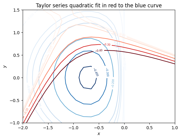

Minimization by gradient descent¶

Example 1 : minimization by gradient descent¶

Find the minimizer of $f (\bfx) = 0.06\exp( 2x_1 +x_2) + 0.05\exp(x_1−2 x_2) + \exp(−x_1)$ .

In vector form we can write it as:

f (\bfx) = 0.06\exp( [2, 1] \bfx ) + 0.05\exp([1, -2] \bfx) + \exp([-1, 0] \bfx)

(32)

\nabla_\bfx^\top f(\bfx) = 0.06\exp( [2, 1] \bfx )[2, 1] + 0.05\exp([1, -2] \bfx)[1, -2] + \exp([-1, 0] \bfx) [-1, 0]

(33)

Algorithm 9.3 Gradient descent method.

given a starting point $\bfx \in \text{dom}{f}$ .

repeat

Choose step size $\alpha_t$
Update. $\bfx := \bfx - \alpha_t \nabla f(\bfx)$

until stopping criterion is satisfied.

# Define the function
def f(x):
    return (0.06 * np.exp(x @ [2, 1]) 
            + 0.05* np.exp(x @ [1, -2]) 
            + np.exp(x @ [-1, 0]))

# Compute its derivative, the gradient function
def grad_f(x):    
    coeff1 = np.array([2, 1])
    coeff2 = np.array([1, -2])
    coeff3 = np.array([-1, 0])
    # Slicing using None, increases the dimension by 1.
    # 
    return (0.06 * np.exp(x @ coeff1)[..., None] * coeff1
            + 0.05 * np.exp(x @ coeff2)[..., None] * coeff2
            + np.exp(x @ coeff3)[..., None] * coeff3)


assert check_numerical_jacobian(f, grad_f)
f(np.zeros((2,))), grad_f(np.zeros((2,)))

(np.float64(1.11), array([-0.83, -0.04]))

def plot_gradients(func, gradfunc):
    x, y = np.mgrid[-3:3:21j,
                    -3:3:21j]
    bfx = np.concatenate((x[..., None], y[..., None]), axis=-1)
    f = func(bfx)
    dfdx = gradfunc(bfx)
    fig, ax = plt.subplots()
    ctr = ax.contour(x, y, np.log(f), 20, cmap='Blues_r')
    ax.quiver(bfx[..., 0], bfx[..., 1], dfdx[..., 0], dfdx[..., 1])
    ax.set_xlabel('$x$')
    ax.set_ylabel('$y$')
    ax.axis('equal')
    plt.show()

plot_gradients(f, grad_f)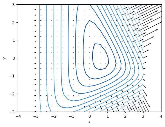

# Implement the gradient descent algorithm
def minimize(x0, f, grad_func, alpha_t=0.2, maxiter=100):
    t = 0
    xt = x0
    grad_f_t = grad_func(xt)
    list_of_xts, list_of_fs = [xt], [f(xt)] # for logging
    while np.linalg.norm(grad_f_t) > 1e-4: # <-- Check for convergence
        xt = xt - alpha_t * grad_f_t # <-- Main update step
        grad_f_t = grad_func(xt) # Compute the next gradient
        
        if t >= maxiter:  # Failsafe, if the algorithm does not converge
            break
        else:
            t += 1
        list_of_xts.append(xt) # for logging
        list_of_fs.append(f(xt)) # for logging
    
    return xt, list_of_xts, list_of_fs

x0 = np.array([-2, 2])
#x0 = np.random.rand(2,2) * 4 - 2
OPTIMAL_X, list_of_xts, list_of_fs = minimize(x0,
                                              f, grad_f, 
                                              alpha_t=0.2,
                                              maxiter=1000)

fig, ax = plt.subplots()
ax.plot(list_of_fs)
ax.set_xlabel('t')
ax.set_ylabel('loss')
plt.show()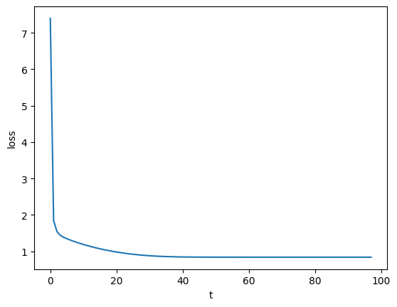

from matplotlib import animation, rc
rc('animation', html='jshtml')

class Anim:
    def __init__(self, fig, ax, func):
        self.fig = fig
        self.ax = ax
        x, y = np.mgrid[-3:3:21j,
                        -3:3:21j]
        bfx = np.concatenate((x[..., None], y[..., None]), axis=-1)
        f = func(bfx)
        self.ctr = self.ax.contour(x, y, np.log(f), 20, cmap='Blues_r')
        self.ax.set_xlabel('x')
        self.ax.set_ylabel('y')
        #self.ax.clabel(self.ctr, self.ctr.levels, inline=True, fontsize=6)
        self.list_of_xs = []
        self.list_of_ys = []
        self.line2, = self.ax.plot([], [], 'r*-')

        
    def anim_init(self):
        return (self.line2,)
        
    def update(self, xt):
        self.list_of_xs.append(xt[0])
        self.list_of_ys.append(xt[1])
        self.line2.set_data(self.list_of_xs, self.list_of_ys)
        return self.line2,
    
fig, ax = plt.subplots()        
a = Anim(fig, ax, f)
animation.FuncAnimation(fig, a.update, frames=list_of_xts[::5],
                        init_func=a.anim_init, blit=True, repeat=False)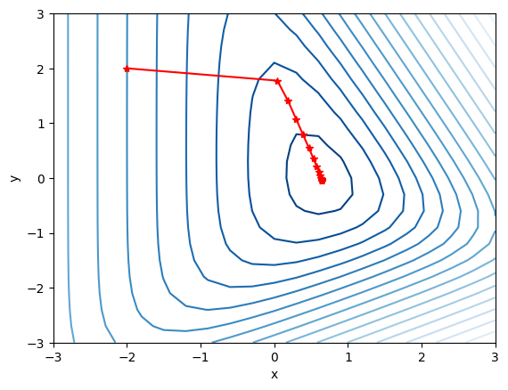

Loading...

# The learning rate can be sensitive to the starting points. 
# Observe the behavior for different starting points
# For different starting points you might need different learning rate scheme

x0 = np.random.rand(2) * 6 - 3
OPTIMAL_X, list_of_xts, list_of_fs = minimize(x0,
                                              f, grad_f, 
                                              alpha_t=0.2,
                                              maxiter=200)
fig, ax = plt.subplots()        
a = Anim(fig, ax, f)
animation.FuncAnimation(fig, a.update, frames=list_of_xts[::10],
                        init_func=a.anim_init, blit=True, repeat=False)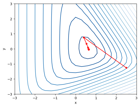

Loading...

Homework (ContinuousOptimization): Problem 1¶

(20 marks)

Following the example above, implement your own gradient descent algorithm that minimizes the following function (50 marks),

f(\bfx) = x_1 \exp(-(x_1^2 + x_2^2))

(34)

Test your algorithm with the starting points of $\bfx_0 = \begin{bmatrix} -1 \\ 1\end{bmatrix}$ and $\bfx_0 = \begin{bmatrix} -1 \\ -1\end{bmatrix}$ and learning rate of $\alpha_t = 0.25$ .

x0 = np.array([-1, 1])


def f(x):
    # YOUR CODE HERE
    raise NotImplementedError()

def grad_f(x):
    # YOUR CODE HERE
    raise NotImplementedError()


## Throw error if grad_f is wrong
assert check_numerical_jacobian(f, grad_f)

# Implement the gradient descent algorithm
def minimize(x0, f, grad_func, alpha_t=0.2, maxiter=100):
    t = 0
    xt = x0
    grad_f_t = grad_func(xt)
    list_of_xts, list_of_fs = [xt], [f(xt)] # for logging
    while np.linalg.norm(grad_f_t) > 1e-4: # <-- Check for convergence
        # 1. Update xt using gradient descent update
        # 2. Compute grad_f_t with new xt
        # YOUR CODE HERE
        raise NotImplementedError()
        if t >= maxiter:  # Failsafe, if the algorithm does not converge
            break
        else:
            t += 1
        list_of_xts.append(xt) # for logging
        list_of_fs.append(f(xt)) # for logging
    
    return xt, list_of_xts, list_of_fs


OPTIMAL_X, list_of_xts, list_of_fs = minimize(x0,
                                              f, grad_f, 
                                              alpha_t=0.25,
                                              maxiter=200)

class Anim:
    def __init__(self, fig, ax, func):
        self.fig = fig
        self.ax = ax
        x, y = np.mgrid[-2:1:21j,
                        -1:1:21j]
        bfx = np.concatenate((x[..., None], y[..., None]), axis=-1)
        f = func(bfx)
        self.ctr = self.ax.contour(x, y, f, 
                                   levels=[-4e-1, -3e-1, -2e-1, -1e-1, -7e-2, -5e-2, -1e-2, -1e-3, 0, 1e-3], 
                                   cmap='Blues_r')
        self.ax.set_xlabel('x')
        self.ax.set_ylabel('y')
        #self.ax.clabel(self.ctr, self.ctr.levels, inline=True, fontsize=6)
        self.list_of_xs = []
        self.list_of_ys = []
        self.line2, = self.ax.plot([], [], 'r*-')

        
    def anim_init(self):
        return (self.line2,)
        
    def update(self, xt):
        self.list_of_xs.append(xt[0])
        self.list_of_ys.append(xt[1])
        self.line2.set_data(self.list_of_xs, self.list_of_ys)
        return self.line2,
    
    
fig, ax = plt.subplots()        
a = Anim(fig, ax, f)
anim1 = animation.FuncAnimation(fig, a.update, frames=list_of_xts[::10],
                                init_func=a.anim_init, blit=True, repeat=False)
anim1

---------------------------------------------------------------------------
NotImplementedError                       Traceback (most recent call last)
Cell In[13], line 14
     10     raise NotImplementedError()
     13 ## Throw error if grad_f is wrong
---> 14 assert check_numerical_jacobian(f, grad_f)
     16 # Implement the gradient descent algorithm
     17 def minimize(x0, f, grad_func, alpha_t=0.2, maxiter=100):

Cell In[4], line 55, in check_numerical_jacobian(f, jac_f, nD, **kwargs)
     53 def check_numerical_jacobian(f, jac_f,  nD=2, **kwargs):
     54     x = np.random.rand(nD)
---> 55     num_jac = numerical_jacobian(f, x, **kwargs)
     56     return np.allclose(num_jac, jac_f(x), atol=1e-06, rtol=1e-4)

Cell In[4], line 47, in numerical_jacobian(f, x, h)
     45 eye = np.eye(n)
     46 x_plus_dx = x + h * eye # n x n
---> 47 num_jac = (f(x_plus_dx) - f(x)) / h # limit definition of the formula # n x m
     48 if num_jac.ndim >= 2:
     49     num_jac = num_jac.swapaxes(-1, -2) # m x n

Cell In[13], line 6, in f(x)
      4 def f(x):
      5     # YOUR CODE HERE
----> 6     raise NotImplementedError()

NotImplementedError:

assert np.allclose(OPTIMAL_X, [-7.07e-01,  1.06e-04], atol=1e-3, rtol=1e-2)

x0 = np.array([-1, -1])
# Repeat minmimization with a different starting point x0
# YOUR CODE HERE
raise NotImplementedError()

assert np.allclose(OPTIMAL_X, [-7.07e-01,  1.06e-04], atol=1e-3, rtol=1e-2)