Hessians - Neural Networks

Recall Linear Least square regression¶

\begin{align} \mathbf{0}^\top &= \frac{\p }{\p \bfm} ( \bfy^\top\bfy + \bfm^\top \bfX^\top \bfX \bfm - 2\bfy^\top \bfX \bfm)\\ &= 2 {\bfm^*}^\top \bfX^\top \bfX - 2\bfy^\top \bfX \end{align}

(1)

This gives us the solution

\bfm^* = (\bfX^\top \bfX)^{-1} \bfX^\top \bfy

(2)

The symbol $\bfV^{-1}$ is called inverse of matrix $\bfV$ .

The term $(\bfX^\top \bfX)^{-1} \bfX^\top$ is also called the pseudo-inverse of a matrix $\bfX$ , denoted as $\bfX^\dagger$ .

%%writefile saltconcentration.tsv
#Observation	SaltConcentration	RoadwayArea
1	3.8	0.19
2	5.9	0.15
3	14.1	0.57
4	10.4	0.4
5	14.6	0.7
6	14.5	0.67
7	15.1	0.63
8	11.9	0.47
9	15.5	0.75
10	9.3	0.6
11	15.6	0.78
12	20.8	0.81
13	14.6	0.78
14	16.6	0.69
15	25.6	1.3
16	20.9	1.05
17	29.9	1.52
18	19.6	1.06
19	31.3	1.74
20	32.7	1.62

Overwriting saltconcentration.tsv

# numpy can import text files separated by seprator like tab or comma
import numpy as np
salt_concentration_data = np.loadtxt("saltconcentration.tsv")

n = salt_concentration_data.shape[0]
bfx = salt_concentration_data[:, 2:3]
bfy = salt_concentration_data[:, 1]
bfX = np.hstack((bfx, np.ones((bfx.shape[0], 1))))
bfX

array([[0.19, 1.  ],
       [0.15, 1.  ],
       [0.57, 1.  ],
       [0.4 , 1.  ],
       [0.7 , 1.  ],
       [0.67, 1.  ],
       [0.63, 1.  ],
       [0.47, 1.  ],
       [0.75, 1.  ],
       [0.6 , 1.  ],
       [0.78, 1.  ],
       [0.81, 1.  ],
       [0.78, 1.  ],
       [0.69, 1.  ],
       [1.3 , 1.  ],
       [1.05, 1.  ],
       [1.52, 1.  ],
       [1.06, 1.  ],
       [1.74, 1.  ],
       [1.62, 1.  ]])

bfm = np.linalg.inv(bfX.T @ bfX) @ bfX.T @ bfy
print(bfm)
bfm, *_ = np.linalg.lstsq(bfX, bfy, rcond=None)
print(bfm)

[17.5466671   2.67654631]
[17.5466671   2.67654631]

import matplotlib.pyplot as plt
m = bfm.flatten()[0]
c = bfm.flatten()[1]

# Plot the points
fig, ax = plt.subplots()
ax.scatter(salt_concentration_data[:, 2], salt_concentration_data[:, 1])
ax.set_xlabel(r"Roadway area $\%$")
ax.set_ylabel(r"Salt concentration (mg/L)")
x = salt_concentration_data[:, 2]
y = m * x + c
# Plot the points
ax.plot(x, y, 'r-') # the line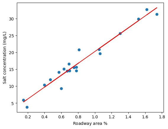

Second derivative aka Hessians¶

Geometry of second derivative¶

import matplotlib.pyplot as plt
plt.rcParams.update({
    "text.usetex": False # turns on math latex rendering in matplotlib
})

x = np.linspace(-10, 10, 100)
fig, ax = plt.subplots(1, 3, figsize=(9, 3))
ax[0].plot(x, x**2, 'r', label=r'$f(x)=x^2$')
ax[0].plot(x, 2*x, 'b', label=r'$\frac{df(x)}{dx}$')
ax[0].set_xlabel('x')
ax[0].legend()

ax[1].plot(x, -x**2, 'r', label=r'$f(x)=-x^2$')
ax[1].plot(x, -2*x, 'b', label=r'$\frac{df(x)}{dx}$')
ax[1].set_xlabel('x')
ax[1].legend()


ax[2].plot(x, x**3, 'r', label=r'$f(x)=x^3$')
ax[2].plot(x, -3*x**2, 'b', label=r'$\frac{df(x)}{dx}$')
ax[2].set_xlabel('x')
ax[2].legend()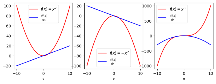

Second derivatives in 2 dimension¶

$f(x, y) = 2x^2 + 4y^2 - xy - 6x - 8y + 6$
$f(x, y) = - 2x^2 - 4y^2 + xy + 6x + 8y + 6$
$f(x, y) = 2x^2 - 4y^2 - xy - 6x + 8y + 6$

Example 1:

f(x, y) = 2x^2 + 4y^2 - xy - 6x - 8y + 6

(3)

\begin{align} f([x, y]) = \begin{bmatrix}x & y \end{bmatrix} \begin{bmatrix}2 & -1/2\\ -1/2 & 4\end{bmatrix} \begin{bmatrix} x \\ y \end{bmatrix} + \begin{bmatrix} - 6 & - 8 \end{bmatrix} \begin{bmatrix} x \\ y \end{bmatrix} + 6 \end{align}

(4)

Example 2:

f(x, y) = - 2x^2 - 4y^2 + xy + 6x + 8y + 6

(5)

\begin{align} f([x, y]) = \begin{bmatrix}x & y \end{bmatrix} \begin{bmatrix}-2 & 1/2\\ 1/2 & -4\end{bmatrix} \begin{bmatrix} x \\ y \end{bmatrix} + \begin{bmatrix} 6 & 8 \end{bmatrix} \begin{bmatrix} x \\ y \end{bmatrix} + 6 \end{align}

(6)

Example 3:

f(x, y) = 2x^2 - 4y^2 - xy - 6x + 8y + 6

(7)

\begin{align} f([x, y]) = \begin{bmatrix}x & y \end{bmatrix} \begin{bmatrix}2 & -1/2\\ -1/2 & -4\end{bmatrix} \begin{bmatrix} x \\ y \end{bmatrix} + \begin{bmatrix} - 6 & 8 \end{bmatrix} \begin{bmatrix} x \\ y \end{bmatrix} + 6 \end{align}

(8)

import plotly.graph_objects as go
import numpy as np
import matplotlib.pyplot as plt
def plot_surface(func):
    x, y = np.mgrid[-20:20:21j,
                    -20:20:21j]
    f =  func(x, y)

    print(f.shape, x.shape, y.shape)
    fig = go.Figure(data=[go.Surface(z=f, x=x, y=y)])
    fig.update_traces(contours_z=dict(show=True, usecolormap=True,
                                      highlightcolor="limegreen", project_z=True))
    fig.show()

Example 1:

f(x, y) = 2x^2 + 4y^2 - xy - 6x - 8y + 6

(9)

f([x, y]) = \begin{bmatrix}x & y \end{bmatrix} \begin{bmatrix}2 & -1/2\\ -1/2 & 4\end{bmatrix} \begin{bmatrix} x \\ y \end{bmatrix} + \begin{bmatrix} - 6 & - 8 \end{bmatrix} \begin{bmatrix} x \\ y \end{bmatrix} + 6

(10)

def f(x, y):
    return 2*x**2 + 4*y**2 - x*y - 6*x - 8*y  + 6

def f_vec(x, y):
    # x is n x n and y is n x n
    xn = x[..., None] # n x n x 1
    yn = y[..., None] # n x n x 1
    vecx = np.concatenate([xn, yn], axis=-1) # n x n x 2
    vecx_col_vec = vecx[..., None] # n x n x 2 x 1
    vecx_row_vec = vecx[..., None, :] # n x n x 1 x 2
    A = np.array([[2, -0.5],
                  [-0.5, 4]]) # 2 x 2
    b = np.array([-6, -8]) # 2
    c = 6
    print("Minima at, ", -np.linalg.inv(A + A.T) @ b)
    quad  = (vecx_row_vec @ A @ vecx_col_vec).squeeze(-1).squeeze(-1)
    return quad + vecx @ b + c

plot_surface(f_vec)

Minima at,  [1.80645161 1.22580645]
(21, 21) (21, 21) (21, 21)

Loading...

f(x, y) = - 2x^2 - 4y^2 + xy - 6x - 8y + 6

(11)

def f(x, y): return - 2*x**2 - 4*y**2 + x*y + 6*x + 8*y  + 6

def f_vec(x, y):
    # x is n x n and y is n x n
    xn = x[..., None] # n x n x 1
    yn = y[..., None] # n x n x 1
    vecx = np.concatenate([xn, yn], axis=-1) # n x n x 2
    vecx_col_vec = vecx[..., None] # n x n x 2 x 1
    vecx_row_vec = vecx[..., None, :] # n x n x 1 x 2
    A = np.array([[-2, 0.5],
                  [0.5, -4]]) # 2 x 2
    b = np.array([6, 8]) # 2
    c = 6
    print("Maxima at, ", -np.linalg.inv(A + A.T) @ b)
    quad  = (vecx_row_vec @ A @ vecx_col_vec).squeeze(-1).squeeze(-1)
    return quad + vecx @ b + c
plot_surface(f_vec)

Maxima at,  [1.80645161 1.22580645]
(21, 21) (21, 21) (21, 21)

Loading...

f(x, ) = 2x^2 - 4y^2 - xy - 6x - 8y + 6

(12)

def f(x, y): return  2*x**2 - 4*y**2 - x*y - 6*x + 8*y  + 6
plot_surface(f)

(21, 21) (21, 21) (21, 21)

Loading...

Second derivative in n-D : Hessian matrix¶

Hessian matrix of a scalar-valued vector function $f: \bbR^n \to \bbR$ is defined as the following arrangement of second derivatives,

\calH f(\bfx) = \begin{bmatrix} \pfxixj11 & \pfxixj12 & \dots & \pfxixj1n \\ \pfxixj21 & \pfxixj22 & \dots & \pfxixj2n \\ \vdots & \vdots & \ddots & \vdots \\ \pfxixj{n}1 & \pfxixj{n}2 & \dots & \pfxixj{n}n \\ \end{bmatrix}

(13)

It is sometimes also written as $\nabla^2 f(\bfx)$ , and hessian can be computed by taking the Jacobian of the gradient,

\calH f(\bfx) = \calJ^\top ( \nabla f(\bfx) )

(14)

If the second partial derivatives are continuous then the Hessian matrix is symmetric.

Find the Hessian of the general quadratic form,¶

f(\bfx) = \bfx^\top A \bfx + \bfb^\top \bfx + c

(15)

Find the gradient of $f(\bfx)$

\nabla^\top f(\bfx) = \bfx^\top (A + A^\top) + \bfb^\top

(16)

Take transpose

\nabla f(\bfx) = (A + A^\top)\bfx + \bfb

(17)

Find the Jacobian of the gradient

\calJ^\top_\bfx \nabla f(\bfx) = (A + A^\top)

(18)

Homework (Hessians): Problem 1¶

(10 marks)

Find the Hessian of the quadratic function that we got as the objective function in linear regression,

R(\bfm) = \bfy^\top \bfy - 2\bfy^\top \bfX \bfm + \bfm^\top \bfX^\top \bfX \bfm,

(19)

where $\bfy \in \bbR^n$ , $\bfm \in \bbR^2$ , and $\bfX \in \bbR^{n \times 2}$ .

Find the Hessian $\calH_\bfm R(\bfm)$ with respect to $\bfm$ .

Positive definite, Negative definite and Indefinite¶

Positiive definite¶

A square matrix $A \in \bbR^{n \times n}$ is called positive definite if for all $\bfx \in \bbR^n$ , $\bfx^\top A \bfx \succ 0$ .

Negative definite¶

A square matrix $A \in \bbR^{n \times n}$ is called negative definite if for all $\bfx \in \bbR^n$ , $\bfx^\top A \bfx \prec 0$ .

Indefinite¶

A square matrix $A \in \bbR^{n \times n}$ is called indefinite if it is neither positive definite nor negative definite.

Eigenvalues and Eigen vectors¶

Eigen values $\lambda \in \bbR$ and eigen vector $\bfv \in \bbR^n$ of a given matrix $\bfA$ are the solutions of the equation,

A \bfv = \lambda \bfv

(20)

You might have solved for eigen values and eigen vectors using the equation

(A - \lambda I_n) \bfv = 0

(21)

whose solution is given by,

\det(A - \lambda I_n) = 0

(22)

Contour Plots¶

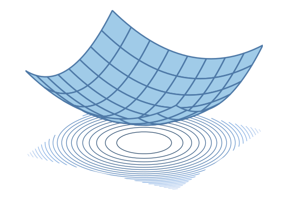
def plot_contour(func):
    x, y = np.mgrid[-20:20:21j,
                    -20:20:21j]
    bfx = np.array([x, y])
    f = func(x,y)

    plt.contour(x, y, f, 20, cmap='Blues_r')
    plt.plot([1.8], [1.2], 'ro') 
    plt.text(1.8+1, 1.2, '$x^*$', color='r')
    plt.xlabel('$x$')
    plt.ylabel('$y$')
    plt.show()

def f(x, y): return  2*x**2 + 4*y**2 - x*y - 6*x - 8*y  + 6
plot_contour(f)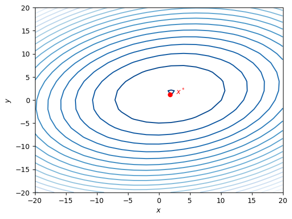

But how about other kinds of functions say:

\arg~\min_x f(x) = x \exp(-(x^2 + y^2))

(23)

def plot_contour(func):
    x, y = np.mgrid[-2:2:201j,
                    -2:3:201j]
    f = func(x,y)

    ctr = plt.contour(x, y, f, 10, cmap='Blues_r')
    plt.clabel(ctr, ctr.levels, inline=True, fontsize=6)
    plt.show()

def f(x,y): return  x * np.exp(-(x**2 + y**2))
plot_contour(f)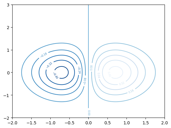

def plot_surface_3d(func):
    x, y = np.mgrid[-2:2:201j,
                    -2:3:201j]
    f = func(x,y)
    fig = go.Figure(data=[go.Surface(z=f, x=x, y=y,
                                    contours = {
                                        "x": {"start": -2, "end": 2, "size": 0.2},
                                        "z": {"start": -2, "end": 2, "size": 0.2}
                                    },
                                    )])
    fig.update_traces(contours_z=dict(show=True, usecolormap=True, project_z=True))
    fig.show()

plot_surface_3d(f)

Loading...

Geometry of eigen vectors and eigen values¶

Example 1:

f(x, y) = 2x^2 + 4y^2 - xy - 6x - 8y + 6

(24)

f([x, y]) = \begin{bmatrix}x & y \end{bmatrix} \begin{bmatrix}2 & -1/2\\ -1/2 & 4\end{bmatrix} \begin{bmatrix} x \\ y \end{bmatrix} + \begin{bmatrix} - 6 & - 8 \end{bmatrix} \begin{bmatrix} x \\ y \end{bmatrix} + 6

(25)

def f(x, y):
    return 2*x**2 + 4*y**2 - x*y - 6*x - 8*y  + 6

def f_vec(x, y):
    # x is n x n and y is n x n
    xn = x[..., None] # n x n x 1
    yn = y[..., None] # n x n x 1
    vecx = np.concatenate([xn, yn], axis=-1) # n x n x 2
    vecx_col_vec = vecx[..., None] # n x n x 2 x 1
    vecx_row_vec = vecx[..., None, :] # n x n x 1 x 2
    A = np.array([[2, -0.5],
                  [-0.5, 4]]) # 2 x 2
    b = np.array([-6, -8]) # 2
    c = 6
    print("Minima at, ", -np.linalg.inv(A + A.T) @ b)
    quad  = (vecx_row_vec @ A @ vecx_col_vec).squeeze(-1).squeeze(-1)
    return quad + vecx @ b + c

x, y = np.mgrid[-4:4:201j,
                -4:4:201j]
fvals = f(x,y)


A = np.array([[2, -0.5],
              [-0.5, 4]]) # 2 x 2

b = np.array([-6, -8]) # 2
minpt = -np.linalg.inv(A + A.T) @ b
ctr = plt.contour(x, y, fvals, 10, cmap='Blues_r')
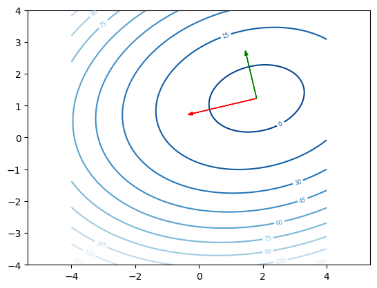
lambdas, V = np.linalg.eigh(A+A.T)
v1 = V[:, 0]
v2 = V[:, 1]
plt.arrow(minpt[0], minpt[1], 4*v1[0]/np.sqrt(lambdas[0]),  4*v1[1] / np.sqrt(lambdas[0]), color='r', head_width=0.1)
plt.arrow(minpt[0], minpt[1], 4*v2[0]/np.sqrt(lambdas[1]),  4*v2[1] / np.sqrt(lambdas[1]), color='g', head_width=0.1)
plt.clabel(ctr, ctr.levels, inline=True, fontsize=6)
plt.axis('equal')
plt.show()