Optimization perspective is not enough¶

So far in this course, we stuck to an optimization perspective on Machine Learning. We identified the following steps:

1. Collecting a training dataset $\calD = \{ (\bfx_1, \bfy_1), \dots, (\bfx_n, \bfy_n) \}$

2. Selecting a model $\hat{\bfy} = f(\bfx; \bfw)$ with weights (also called the parameters) $\bfw$.

3. Selecting a loss function $l(\bfy_i, \hat{\bfy}_i)$

4. Training: Minimizing the total or average loss function to find the optimal weights

5. For a new input $\bfx^* \notin \calD$, use $\hat{\bfy}^* = f(\bfx^*; \bfw^*)$ as the prediction.

For linear models (or other “simple” models) this perspective works fine. However, in general it does not.

Question Imagine you are designing a pedestrian detector (input: image, output: a box around all pedestrians in the image) for an autonomous car (or a face detector for your ring-camera based security system). You collect a training dataset of pedestrians in Iceland and then try to deploy it in India.

• How well is your pedestrian detector likely to work? Very good, very bad, okayish.

• Why?

• How would describe the reason mathematically?

Independent and Identically distributed¶

A random variable $Z_1$ is said to be independent from random variable $Z_2$, denoted as $Z_1 \perp Z_2$ if either of the three equivalent conditions are met:

1. $\bbP(Z_1, Z_2) = \bbP(Z_1) \bbP(Z_2)$

2. $\bbP(Z_1 | Z_2) = \bbP(Z_1)$

3. $\bbP(Z_2 | Z_1) = \bbP(Z_2)$

In typical machine learning, we want the data samples to be Independent and Identically Distributed, in short the i.i.d assumption.

Maximum Likelihood estimation¶

The optimization perspective can be related to maximum likelihood estimation under the iid (Independent and Indentically distributed) assumpotion.

Let the $\bfx_i$ and $y_i$ be random vectors for all $i$. Model the probability distribution as a negative log of the loss function:

If the samples are IID, then we can write the probability of the entire dataset as products of sample probabilities

A product of exponents is the summation of their powers,

Denote

Minimizing the loss is same as maximizing the probability $P(\calD|\bfW)$.

No free lunch theorem¶

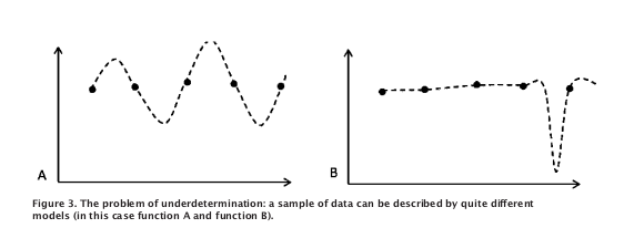
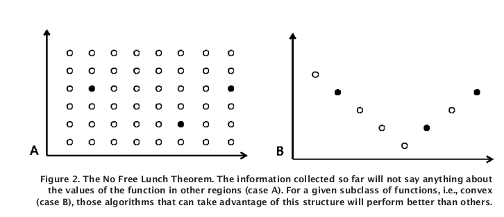
In the era of so much machine learning hype it is important to look back at David Wolpert’s No free lunch theorems. ECE590 students must read Wolpert’s 1996 paper “The Lack of A Priori Distinctions Between Learning Algorithms” and mark the terms, symbols and concepts that do not make sense.

Expectation vs Mean¶

Given i.i.d. random variables $Z_1, Z_2, ... Z_n$ with distribution $\bbP(.)$, write the mathematical definition for the mean and that of the expectation. What is the difference?

Question:¶

What is the diference between Empirical risk and Expected risk?

Answer:¶

Empirical risk is the average loss over the dataset while Expected risk is the expectation of the loss when the inputs and outputs are treated as random variables.

For example, if a dataset $\calD = \{(\bfx_1, y_1), \dots, (\bfx_n, y_n)\}$ with $\bfx_i \in \bbR^n$ and $y_i \in \bbR$ is given and the model $f(\bfx_i; \bfW)$ predicts labels $\hat{h}_i = f(\bfx_i; \bfW)$. Then the empirical risk is the average loss over the dataset samples,

On the other hand to compute Expected risk, we assume that the dataset $\calD$ was independently sampled (IID assumption) from a distribution $\bbP_{X,Y}$ where the input $\bfx_i$ is an instance of random variable $X$ and $y_i$ is an instance of random variable $Y$.

where $\hat{Y} = f(X; \bfW)$.

If $X$ and $Y$ are continous random variables, then the expectation is the weighted integraal over all possible values of values of $X$ and $Y$ weighted by the joint probability density function (PDF) of $X$ and $Y$.

where $\hat{y} = f(x; \bfW)$ and $\Omega_X$ and $\Omega_Y$ is the sample space for $X$ and $Y$.

Generalization gap bounds in Machine Learning¶

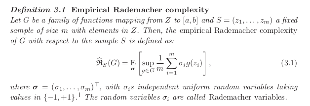
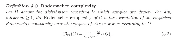
There are many generalization gap bounds in machine learning, often studied under Machine Learning theory; Probably Approximatly Correct (PAC) theory. Mohri 2012, Foundations of Machine Learning is an excellent book to learn more about it.

If the loss $l(.,.)$ is between [0, 1], then for any $\delta > 0$ with Probability at least $1-\delta$, we have

where Rademacher Complexity is defined as

Bayes Rule¶

Question:¶

Given two random variables $X$ and $Y$ specify the relationship between $P(X|Y)$ and $P(Y|X)$ using Bayes rule?

Answer¶

Question:¶

Using CIFAR 10 dataset $\calD$ you want to find your neural network with weights $\bfW$. Define Prior, Likelihood and Posterior in terms of the weights $\bfW$ and data $\calD$. Write Bayes rule to determin posterior from likehood and prior.

Answer:¶

• Prior is $P(\bfW)$ i.e. the probability of weights $\bfW$ before we have seen the dataset.

• Likelihood is $P(\calD|\bfW)$ i.e. the probability of observing the dataset once if we pick a particular choice of weighs $\bfW$.

• Posterior is $P(\bfW|\calD)$ i.e the probability of chosing weights given the dataset $\calD$.

By Bayes rule, we have:

Question:¶

How can regularization can be interpretted as an application of the Bayes theorem?

Given the dataset $\calD = \{ (\bfx_1, y_1), \dots, (\bfx_n, y_n) \}$, a model $\hat{y}_i = f(\bfx_i; \bfW)$, a regularizer $R(\bfW)$ and a loss function $l(y_i, \hat{y}_i)$, show that the following optimization problem can be interpreted as maximum-a-posteriori estimation. In the process show that for the interpretation, we need the IID (independently, identically distributed) assumption over the dataset. List any other assumptions that you need for the interpretation.

where $\lambda$ is some positive constant that balances between the loss function and the regularizer.

Answer:¶

Let the $\bfx_i$ and $y_i$ be random vectors for all $i$. Model the probability distribution as a negative log of the loss function:

If the samples are IID, then we can write the probability of the entire dataset as products of sample probabilities

A product of exponents is the summation of their powers,

Denote

The original optimization problem can be written as:

Taking negative exponent on both sides turns the problem into a maximization problem because $\exp(-y)$ is a monotonically decreasing function.

The first term is the same as maximizing the likelihood $P(\calD|\bfW)$. If we interpret the second term as a prior:

then we can rewrite the original optimization problem as

By Bayes theorem $P(\calD|\bfW) P(\bfW) = P(\bfW|\calD)P(\calD)$, hence we can write the optimization problem as maximizing the posterior

We can ignore the evidence term $P(\calD)$, because it is independent of $\bfW$ the optimization variable. The original problem reduces to maximizing the posterior, hence maximum a posteriori:

Question:¶

You are doing 0-1 binary classification on the MNIST hand digit classification task. Let detecting the digit 1 be considered the positive class. Using this example, define the terms False negative, False positive, Accuracy, Precision, recall, F1-score.

Answer:¶

• False negative: is the case when the predictor classifies the digit as negative i.e. 0 but it is actually 1.

• False positive: is the case when the predictor classifies the digit as positive i.e. 1 but it is actually 0.

• Accuracy: Total correct classifictions/Total samples .

• Precision: True positives / Predicted positives.

• Recall: True positives / All actual positives.

Question:¶

What is a ROC (Receiver Operating characteristics) for a binary classifier? Argue why it lies above the diagonal for any reasonable classifier? Also, argue why it must be concave?

Answer:¶

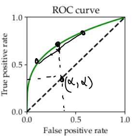
ROC curve is plot between False positive rate (FPR) $P(\hat{Y}(X) = 1| Y=0)$ and True positive rate (TPR) $P(\hat{Y}(X) = 1| Y = 1)$.

ROC curve is always lies above the diagonal because you can construct a trivial classifier that predicts the positive class with probability $\alpha \in (0, 1)$, i.e. $P(\hat{Y} = 1) = \alpha$ without even looking at the input data $X$. This trivial classifier will form the diagonal of the ROC curve with both FPR and TPR being equal to $\alpha$. Any classifier that works better than this trivial classifier will lie above the diagonal.

Why ROC curve is a concave curve

Suppose you are given hyperparameter values on the ROC curve of a classifier such that:

1. The first classifier 1 has true positive rate (TPR) is $P(\hat{Y}_1(X) = 1| Y = 1) = TPR(f_1)$ at given FPR $P(\hat{Y}_1(X) = 1| Y=0) = f_1$ .

2. Similarly second classifier 2 has $FPR = P(\hat{Y}_2(X) = 1| Y = 0) = f_2$, assume it’s TPR is $TPR(f_2)$.

If you pick the classifier $f_1$ randomly with probability $P(\hat{Y} = \hat{Y}_1) = \alpha$ and the other one with probability $P(\hat{Y} = \hat{Y}_2) = 1-\alpha$, and take the output of the picked classifier.

Then you have FPR of this new classifier as $FPR =P(\hat{Y}_1(X) = 1| Y = 0)\alpha + P(\hat{Y}_2(X) = 1| Y = 0)(1-\alpha) = f_1\alpha + f_2(1-\alpha)$. If you get a better TPR than this randomized classifier, the ROC curve will be concave $TPR^*(\alpha f_1 + (1-\alpha) f_2) > \alpha TPR(f_1) + (1-\alpha) TPR(f_2)$.

The definition of concavity: A function $g$ is concave if for all points $y_1$, $y_2$ and all $\alpha \in (0, 1)$ the following condition is true, $g(y_1 \alpha + y_2 (1-\alpha) > g(y_1)\alpha + g(y_2)(1-\alpha)$.

Question:¶

What is the likelihood ratio test for a binary classifier? Is it better or worse than Posterior ratio test?

Answer:¶

For a binary classifier, likelihood is the probability of observing the evidence $\bfx$ given a hypothesis class $y \in \{0, 1\}$,

Likelihood ratio test gives us a classifier that predicts the positive class $y = 1$ if the likelihood ratio exceeds a given threshold $\eta$,

Posterior is the probability of hypothesis class $y$ given an observed evidence $\bfx$,

Let the posterior ratio test be,

Posterior ratio test and likelihood ratio test are equivalent, because the condition for posterior ratio test can be written as likelihood ratio test,

The last condition is the same condition in the likelihood ratio test with $\eta = \frac{\bbP(y=0)}{\bbP(y=1)}\eta_p$.

Submission¶

Make sure you have run all cells in your notebook in order before running the cell below, so that all images/graphs appear in the output. The cell below will generate a zip file for you to submit. Please save before exporting!

Upload the generated zip file to the gradescope autograder