Linear algebra¶

Open in Binder

• Read Chapter 2 of MML Book by Deisenroth et al https://mml-book.github.io/

1. Linear algebra is the study of vectors and certain rules to manipulate vectors.

Equation of a 2D line¶

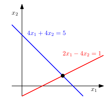
There are two equations of lines

1. $y = m x + c$

2. $a x + b y + c = 0$

What are the advantages or disadvantages of both of those?

A 2D line is the set of all points (x, y) that satisfy the an equation $a x + b y + c = 0$ for given $a, b, c$. For the same line there can be multiple valid parameters $a, b , c$. Either $a$ or $b$ can be zero. But both $a$ and $b$ cannot be zero at the same time.

Ideally the equation of line must be written in the set notation:

This equation is read as: the line $\mathcal{L}$ defined by the paramters $a,b,c$ is the set of all points $(x, y)$ such that it the $x,y$ satisfy the equation $ax + by + c = 0$ and $x$ and $y$ are in the set of all real numbers.

Implicit form¶

Line is a type of curve. Other curves can be parabola, circle etc. Every curve can be represented in implicit form like we did for the line above. In implicit form, the points are constrained by one or more equations to lie on the curve. The equations define a test whether the point lies on the curve or not.

This equation is read as the curve $\calC$ defined by the paramters $p_1, p_2, \dots, p_n$ is the set of all points $(x, y)$ such that it the $x,y$ satisfy the equation $f(x, y; p_1, p_2, \dots, p_n) = 0$ and $x$ and $y$ are in the set of all real numbers.

Take circle with center $(x_0, y_0)$ and radius $r$, as an example. The implicit form is:

Paramteric form of 2D Line¶

A parameteric form defines how the points on the curve are generated from a free paramters. For a line:

This equation is read as: the line $\calL$ defined by the paramters $d_x,d_y,x_0,y_0$ is the set of all points $(d_xr+x_0, d_yr+y_0)$ such that $r$ is any real number.

Take circle with center $(x_0, y_0)$ and radius $r$, as an example. The parameteric form is:

In general, the paramteric form of a curve depend on some free paramters and the points are defined as functions of the free parameters.

Linear system of equations and Matrices¶

The equation

can be written in matrix form as,

In general a system of $m$ equations with $n$ unknowns,

can be written in matrix form as

Or

Vectors¶

We will denote vectors with bold font notations instead of the usualy $\vec{x}$ notation. The arrow notation vectors are sometimes called geometric vectors. We will make no such distinction. The set of all real numbers will be denoted as $\bbR$. The set of all real 2D vectors is written as $\bbR^2$. When we write $\bfx \in \bbR^2$, it means that $\bfx$ is in the set of real 2D vectors, hence a 2D real vector. We will write $\|\bfx\|$ for the magnitude of the vector, and $\bfx \cdot \bfy$ for dot product between two vector $\bfx$ and $\bfy$.

n-D vector¶

A n-D vector is also written as $\bfx \in \bbR^n$ and the vector has $\bfx = [x_1; \dots; x_n]$ $n$ real components. Every vector has a magnitude $\|\bfx\|$ and a direction $\hat{\bfx}$. The magnitude and direction are given by:

The direction vector $\hat{\bfx}$ is a unit vector because its magnitide is one i.e. $\|\hat{\bfx}\| = 1$.

Vector addition¶

Vector addition is element-wise addition

Geometrically the resulting vector can be obtained by triangle law or the parallelogram law.

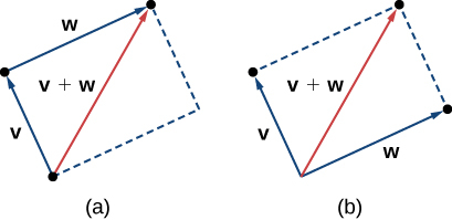
Reference: [1]

Dot product of vectors¶

Dot product of two vectors is a scalar given by sum of element-wise product.

Geometrically, dot product is closely related to the projection. Projection of vector $\bfv$ on $\bfu$ is the dot product of $\bfv$ with the direction of $\bfu$

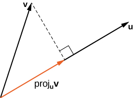
Dot product of vector with itself gives the square of the magnitude $\bfv \cdot \bfv = \|\bfv\|^2$.

Reference: [2]

Matrices¶

Matrices are a group of vectors. A matrix can be obtained by vertical stacking of row (horizontal) vectors or horizontal stacking of column (vertical) vectors. It is common to represent all vectors as column vectors unless specified otherwise, so we consider a matrix $\bfV$ as a horizontal concatenation of column vectors $\bfv_1, \bfv_2, \dots, \bfv_n$. Let each vector be m-dimensional $\bfv_i \in \bbR^m$.

Such a matrix is said to be a $m \times n$ matrix. It is also written as $\bfV \in \bbR^{m \times n}$.

Linear functions¶

What are linear functions?

Definition of Linear combination (2.11 in MML book)¶

Given $m$ vectors $\bfx_1, \bfx_2, \dots, \bfx_m \in \bbR^n$, a linear combination of vectors is defined as, $\mathbf{v} := \alpha_1 \bfx_1 + \alpha_2 \bfx_2 + \dots + \alpha_n \bfx_m$ for every any scalar $\alpha_1, \alpha_2, \dots \alpha_n \in \bbR$

Definition of Linear function¶

A function $f: \mathbb{R}^n \to \mathbb{R}^m$ is linear in $\mathbf{x}$ when

1. $f(\alpha\mathbf{x}) = \alpha f(\mathbf{x})$ for all $\alpha \in \mathbb{R}$ and $\mathbf{x} \in \mathbb{R}^n$

2. $f(\mathbf{x} + \mathbf{y}) = f(\mathbf{x}) + f(\mathbf{y})$ for all $\alpha, \beta \in \mathbb{R}$ and $\mathbf{x}, \mathbf{y} \in \mathbb{R}^n$

The above two properties can be combined in a single test

Examples of linear functions¶

1. $f([x_1, x_2]) = 3x_1 + 2x_2$

2. $f([x_1, x_2, x_3]) = 4(3x_1 + 2x_2) + x_3$

3. $f([x_1, x_2, x_3], [w_1, w_2, w_3]) = w_1x_1 + w_2x_2 + w_3 x_3$

4. $f([x_1, x_2]) = \exp(\log(3x_1 + 3x_2))$

5. $f([x_1, x_2]) = ((3x_1 + 3x_2)^2)^{(1/2)}$

Homework (Linear Models). Problem 1¶

(10 marks) Show that the above functions are linear.

Examples of non-linear functions¶

1. $f([x_1, x_2]) = x_1^2$

2. $f([x_1, x_2]) = x_1^3$

3. $f([x_1, x_2]) = \sin(x_1)$

4. $f([x_1, x_2]) = \exp(x_1)$

5. $f([x_1, x_2]) = \log(x_1)$

Homework (Linear Models). Problem 2¶

(10 marks) Show that the above functions are non-linear.

Properties of Matrices¶

Transpose of a Matrix¶

Transpose of a matrix $\bfV$ (denoted as $\bfV^\top$) is an operation that swaps rows with columns and columns with rows. For example, the transpose of the above matrix will make it a vertical concatenation of row vectors.

If $\bfV \in \bbR^{m \times n}$, then $\bfV^\top \in \bbR^{n \times m}$. The two dimensions get swapped.

Tranpose of a column vector¶

All vectors are also matrices. By convention, all vectors are considered column matrices and hence called column vectors. A n-D vector $\bfv = [v_1; \dots; v_n] \in \bbR^n$ is by convention considered a $n \times 1$ column matrix i.e. $\bfv \in \bbR^{n \times 1}$.

The transpose of a column vector is a row vector

Row vectors are always denoted with a tranpose of their corresponding column vector.

Matrix addition¶

You can add two matrices element-wise.

The matrix addition is commutative $A + B = B + A$

Matrix-scalar product¶

You can multiply matrices with a scalar (a real number)

Matrix scalar product is commutative

Matrix-vector product¶

For those who know dot product, matrix-vector product is best defined as a collection of dot products. Define a matrix $\bfV \in \bbR^{m \times n}$ as a vertical concatenation of $m$ n-dimensional row-vectors $\bfv_1^\top, \dots \bfv_m$

The matrix $\bfV \in \bbR^{m \times n}$ can be multiplied by a n-dimensional column vector $\bfu \in \bbR^{n}$ with the product defined as the vector-wise dot product vertically concatenated to result in another column vector:

When $m = 1$, then $\bfV = \bfv_1^\top$ and the matrix product is $\bfv_1^\top \bfu = \bfv_1 \cdot \bfu$. Dot product between two vectors $\bfv$ and $\bfu$ is also written as $\bfv^\top \bfu$. Going forward we will prefer $\bfv^\top \bfu$ notation for dot product instead of $\bfv \cdot \bfu$.

Matrix-matrix product¶

Matrix-matrix product between two matrices $\bfV \in \bbR^{m \times n}$ and $\bfU \in \bbR^{n \times p}$ can be defined in terms of matrix-vector product by writing $\bfU$ as a horizontal concatenation of $p$ $n$-dimensional column vectors $\bfu_1, \bfu_2, \dots, \bfu_p$.

The result is a horizontal concatenation of matrix-vector products, where the left matrix $\bfV$ gets multiplied with each column vector of right matrix $\bfU$.

Another interpretation is that the matrix-matrix product are all possible dot products between left matrices’ row vectors with right matrices’ column vectors.

Matrix-matrix product or short matrix products do not commute i.e $\bfV \bfU \ne \bfU \bfV$ in general.

Matrix-matrix product does follow distributive property $A(B + C) = AB + AC$.

Identity matrix¶

Square matrix¶

A square matrix is a matrix with number of rows equal to the number of columns.

Inverse of a square matrix¶

A matrix $\bfV^{-1}$ is called the inverse of a square matrix $\bfV$ if $\bfV^{-1} \bfV = \bfV^{-1} = \bfI_n$. The inverse of a square matrix exists only when it is singular i.e the determinant of the matrix is non-zero $\det(\bfV) \ne 0$.

Linearity of matrix multiplication¶

Consider a function $f_A : \bbR^n \to \bbR^m$ defined as

.

Show that the function $f_A$ is linear.

Proof¶

The function $f_A(\bfx)$ is linear if for any $\bfx,\bfy \in \bbR^n$ and $\alpha, \beta \in \bbR$,

Theorem¶

All linear functions of the form $f : \bbR^m \to \bbR^n$ can be written as matrix multplications of the form $f(\bfx) = F \bfx$.

Proof:¶

Consider any given linear function $f : \bbR^m \to \bbR^n$ which is linear. Because of linearity it satisifies $f(\alpha \bfx + \beta \bfy) = \alpha f(\bfx) + \beta f(\bfy)$.

Consider special vectors, called the standard basis vectors, that have only one element as 1 and the rest are 0.

Any vector $\bfx = [x_1, x_2, \dots, x_n]^\top \in \bbR^n$ can be written as a linear combination of standard basis vectors,

$\bfx = x_1 \bfe_1 + x_2 \bfe_2 + \dots + x_n \bfe_n$

Hence the function evaluation at $\bfx$, can also be written as the linear combination of function evaluations at standard basis vectors,

Note that $f(\bfe_1)$, $f(\bfe_2)$, are constants with respect to $\bfx$. So you can arrange them into a constant matrix, independent of $\bfx$,

Theorem¶

Show that composition $f(g(\bfx))$ of two linear functions, $f$ and $g$ is also a linear function.

Homework (Linear Models) Problem 3¶

(10 marks) Proof is left as a homework for the above theorem.

Using vectors for 2D line notation¶

Matplotlib¶

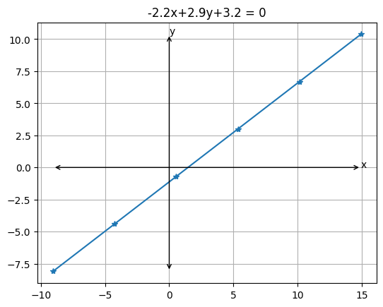
We started from 2D linear models, but we want to work with N-D models where N can be even in thousands or millions. It makes sense to simplify the notation by using vector notation.

Recall that the implicit equation for a line is

We will represent a 2D point (x, y) by a 2D vector $\bfx = [x; y]$ and the parameters $(a, b)$ with weight vector $\bfw = [a; b]$. Let’s compute the dot product between the two newly defined vectors :

The equation of the line under new notation in full its full glory is

Unique line notation¶

Same line $ax + by + c = 0$ can be represented by multiple equations for the same form. This representation of line is not unique. For example, equations $5x + 2y + 10 = 0$ and $10x + 4y + 20 =0$ represent the same line. In general, for any real number $\alpha \ne 0$ all equations $\alpha a x + \alpha b y + \alpha c = 0$ represent the same line. Once can choose an arbitrary non-zero $\alpha$ for making the equation unique.

In vector notation, all non-zero $\alpha \bfw \cdot \bfx + \alpha c = 0$ represent the same line. One good candidate for $\alpha$ is $\alpha = \frac{1}{\|\bfw\|}$, because this changes $\alpha \bfw$ to $\hat{\bfw}$ a unit vector.

where $w_0 = \frac{c}{\|\bfw\|}$.

Geometric interpretaion¶

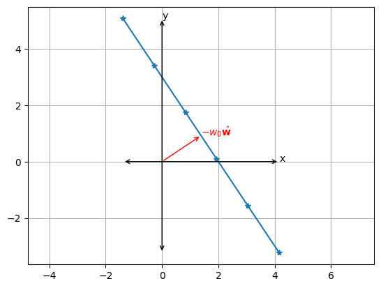
The new equation of the line has a convinient geometric interpretation. Recall that $\hat{\bfw} \cdot \bfx$ is the projection of $\bfx$ on $\hat{\bfw}$. In other words, the equation $\text{proj}_{\hat{\bfw}}\bfx + w_0 = 0$ constrains all vectors on the line to have a constant projection $\text{proj}_{\hat{\bfw}}\bfx = -w_0$.

This means that vector $\hat{\bfw}$ is perpendicular to the line and cuts the line a distance $|w_0|$ from the origin.

Numpy: General Broadcasting Rules¶

When operating on two arrays, NumPy compares their shapes element-wise. It starts with the trailing (i.e. rightmost) dimension and works its way left. Two dimensions are compatible when

1. they are equal, or

2. one of them is 1.

Otherwise a ValueError is raised

Ref: https://numpy.org/doc/stable/user/basics.broadcasting.html

In the following example, both the A and B arrays have axes with length one that are expanded to a larger size during the broadcast operation:

A      (4d array):  8 x 1 x 6 x 1
B      (3d array):      7 x 1 x 5
Result (4d array):  8 x 7 x 6 x 5

Here are some more examples:

A      (2d array):  5 x 4
B      (1d array):      1
Result (2d array):  ?

A      (2d array):  5 x 4
B      (1d array):      4
Result (2d array):  ?

A      (3d array):  15 x 3 x 5
B      (3d array):  15 x 1 x 5
Result (3d array):  

A      (3d array):  15 x 3 x 5
B      (2d array):       3 x 5
Result (3d array):  ?

A      (3d array):  15 x 3 x 5
B      (2d array):       3 x 1
Result (3d array):  ?

Linear regression: review¶

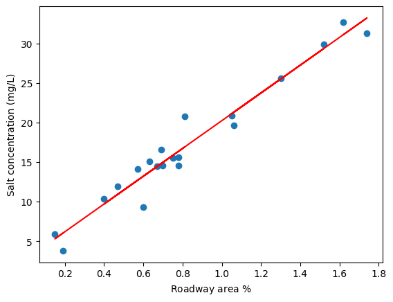
Let’s take the simple linear regression example from STS332 textbook (uploaded on brightspace;page 300; Table 6-1).

“As an illustration, consider the data in Table 6-1. In this table, y is the salt concentration (milligrams/liter) found in surface streams in a particular watershed and x is the percentage of the watershed area consisting of paved roads.”

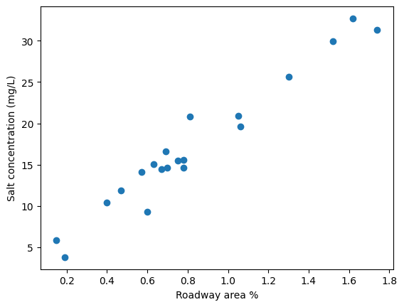
Least squares regression¶

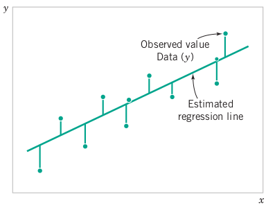
The problem of linear regression is to find a line that “best fits” the given data. That is we want all the points $\{(x_1, y_1), \dots, (x_n, y_n)\}$ to satisfy the equation of the line $y = mx + c$. Since we know that there exists no such line, so we will try to make $y \approxeq mx + c$, by minimizing some error/distance/cost/loss function between $y$ and $mx + c$ for every point $(x_i, y_i)$ in the dataset. The simplest error function that results in nice answers is squared distance:

Then we can minimize the total error to find the line:

Geometrically, this error minimization corresponds to minimizing the stubs in the following figure:

Vectorization of Least square regression¶

Recall that the magnitude of a vector $\|\bfv\| = \sqrt{v_1^2 + v_2^2 + \dots + v_n^n}$ has a similar form to the error function. This suggests that we can define an error vector with the signed error for each data point as it’s elements

Minimizing the total error is same as minimizing the square of error vector magnitude

While we are at at it let us define $\bfx = [x_1; \dots; x_n]$ to denote the vector of all x coordinates of the dataset and $\bfy = [y_1; \dots; y_n]$ to denote y coordinates. Then the error vector is:

where $\mathbf{1}_n$ is a n-D vector of all ones. Finally, we vectorize parameters of the line $\bfm = [m; c]$. We will also need to horizontally concatenate $\bfx$ and $\mathbf{1}_n$. Let’s call the result $\bfX = [\bfx, \mathbf{1}_n] \in \bbR^{n \times 2}$. Now, the error vector looks like this:

Expanding the error magnitude:

Homework (Linear Models): Problem 4¶

(10 marks)

Expand

and show that it is equal to

Our minimization problem in vectorized form is:

This is a quadratic equation in $\bfm$ that can be minimized by equating the derivate to zero.

Two rules of vector derivatives¶

There are two conventions in vector derivatives:

1. Gradient convention

2. Jacobian convention

Gradient convention¶

Under gradient convention the derivative of scalar-valued vector function function $f(\bfx): \bbR^n \to \bbR$ is defined as vertical stacking of element-wise derivatives

Jacobian convention¶

Under gradient convention the derivative of scalar-valued vector function function $f(\bfx): \bbR^n \to \bbR$ is defined as horizontal stacking of element-wise derivatives

For a vector-value vector function $\bff(\bfx): \bbR^n \to \bbR^m$, Jacobian of $\bff(\bfx)$ is the vertical concatentation of gradients transposed, resulting in $m \times n$ matrix

We will use Jacobian convention in this course, because it works nicely with chain rule.

Derivative of a linear function¶

All scalar-valued linear functions of $\bfx$ can be written in the form $f(\bfx) = \bfc^\top \bfx$.

Derivative of a quadratic function¶

All scalar-valued homogeneous quadratic functions of $\bfx$ can be written in the form $f(\bfx) = \bfx^\top \bfA \bfx$.

Homework (Linear Models): Problem 5¶

(10 marks)

Proof of above two derivatives is left as an exercises.

Back to Least square regression¶

This gives us the solution

The symbol $\bfV^{-1}$ is called inverse of matrix $\bfV$.

The term $(\bfX^\top \bfX)^{-1} \bfX^\top$ is also called the pseudo-inverse of a matrix $\bfX$, denoted as $\bfX^\dagger$.