1. Pytorch basics: https://colab.research.google.com/github/wecacuee/ECE490-Neural-Networks/blob/master//notebooks/06-pytorch/NumpyTutorial-Pytorched.ipynb (you should understand basic mathematical operations and broadcasting).

2. Midterm 1 review: https://vikasdhiman.info/ECE490-F25-Neural-Networks/notebooks/review/practice-problems-bank/

3. Proabilistic perspective: https://vikasdhiman.info/ECE490-F25-Neural-Networks/notebooks/prob/probabilisticperspective/

4. Probability problems ( below)

Probability definitions¶

Q1: Define Sample Space¶

Sample space is the set all possible of outcomes of an experiment, denoted by $\Omega$.

For example, For 2-coin tosses the sample space is

For roll of a dice with 6-sides

For weight measurements of an individual, the sample space is the set of all positive real numbers

Q2: Define Event Space¶

An event is the set of outcomes that we might be interested in.

Event space is a set of subsets of the sample space.

or example, For 2-coin tosses the set of all subsets of the sample space in cluding the null set $\{\}$ and the full sample $\Omega$

For weight measurements of an individual, the event space is be the set of all unions and intersections of intervals (open and closed) of sample space (positive real numbers).

Q3: Define Power set¶

The set of all possible subsets of a set $\Omega$ is called a power set and is denoted by $2^{\Omega}$.

For roll of a dice with 6-sides

For discrete sample space, event space is the power set of the sample space.

Q4: Define Probability measure¶

Probability measure is a function $P: \mathcal{F} \to [0, 1]$ that maps from event space to real numbers between $[0, 1]$ and satisfy the following Kolmogorov axioms

1. $P(E) \in [0, 1]$ for all $E \in \mathcal{F}$, where $\mathcal{F}$ is event space

2. $P(\Omega) = 1$, where $\Omega$ is sample space

3. For all disjoint set of events $A_1$, $A_2$ ($A_1 \cap A_2 = \phi$), the probability of union of events is the sum of individual event probabilities:

   $$P(A_1) + P(A_2) = P(A_1 \cup A_2)$$

   (7)

   when $A_1 \cap A_2 = \phi$.

   In general, for a countably infinite set of event $A_1, A_2, \dots A_n \dots \infty$,

   $$P\left(\bigcup_{n=1}^\infty A_n\right) = \sum_{n=1}^\infty P(A_n)$$

   (8)

   when $A_i \cap A_j = \infty$ for all $i \ne j$.

Q5: Define Probability space¶

The triple of sample space $\Omega$, event space $\mathcal{F}$ and a probability measure $P: \mathcal{F} \to [0, 1]$ is called a probability space.

Q6: Define Random variable¶

A random variable is a function $X: \Omega \to \mathbb{Q}$ that maps from sample space $\Omega$ to a space of integers $\mathbb{Z}$ or real numbers $\mathbb{R}$ (in general a measurable space), such that a preimage $X^{-1}(B) \in \Omega$ of any set of numbers $B \in \mathbb{Q}$ exists in the sample space.

For example, a 2-coin toss:

A random variable maps the elements of sample space to a number,

By slight abuse of notation, the random variable also maps events to a set of numbers $X: \mathcal{F} \to B$,

Q7: What is the difference between discrete and continuous random variable¶

Discrete random variable: When the random variable maps the sample space to integers, then the random variable is discrete.

Continuous random variable: When the random variable maps the sample space to real numbers then the random variable is continuous.

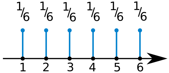
Q8: Define Probability mass function (PMF)¶

For a discrete random variable (RV) the Probability mass function (PMF) is a function that assigns probability value to every discrete value of the random variable, such that

For example, a die roll

PMF is denoted as multiple symbols $P(X=x) = P_X(x) = P(x)$

Q9: Define probability density function (PDF)¶

For a continuous random variable $X: \Omega \to \mathbb{R}$, the probability density function (PDF) is a function $f_X : \mathbb{R} \to [0, \infty)$ such that:

1. $f_X(x) \ge 0$ for all $x \in \mathbb{R}$

2. $\int_{\mathbb{R}} f_X(x) dx = 1$

3. $P(a \le X \le b) = P(X \in [a, b]) = \int_a^b f_X(x) dx$

Q10: Define joint probability mass function¶

Q11: Define joint probability density function¶

For two continuous random variable $X$ and $Y$, the joint probability density function (PDF) is a function $f_{X,Y} : (\mathbb{R}, \mathbb{R}) \to [0, \infty)$ such that:

1. $f_{X,Y}(x, y) \ge 0$ for all $x, y \in \mathbb{R}$

2. $\int_{\mathbb{R}} \int_{\mathbb{R}} f_{X, Y}(x, y) dx dy = 1$

3. $P(a \le X \le b, c \le Y \le d) = P(X \in [a, b], Y \in [c, d]) = \int_c^d\int_a^b f_{X,Y}(x, y) dx dy$

Q12: Define cumulative distribution function¶

A cumulative distribution function (CDF) is $F_X(x)$ is defined as

For a discrete random variable, CDF is the sum of probability mass function

For a continuous random variable, CDF is the integral of probability density function

Q13: Define conditional probability¶

Conditional probability of event $A$ given event $B$ is defined as

when $P(B) \ne 0$.

Q14: State Bayes theorem¶

For any two events, $A$ and $B$

Q15: State Bayes theorem in terms of likelihood, prior, evidence and posterior¶

For an observable event $D$ and a hidden event $\theta$, the posterior $P(\theta|D)$ can be estimated using Bayes theorem in terms of likelihood $P(D|\theta)$, prior $P(\theta)$ and evidence $P(D)$ as

Q16: Define statistical independence¶

Two random variables $X$ and $Y$ are said to be independent, denoted as $X \perp Y$ if any of the following equivalent condition hold for all $x, y$ :

1. $$P(X = x, Y = y) = P(X = x) P(Y = y)$$

   (22)
2. $$P(X = x| Y = y) = P(X = x)$$

   (23)
3. $$P(Y = y| X = x) = P(Y = y)$$

   (24)

Q17: Define conditional independence¶

Two random variables $X$ and $Y$ are said to be conditionally independent given random variable $Z$, denoted as $X \perp Y | Z$ if for all $x, y, z$ :

Q18: Identically independently distributed (IID)¶

The random variables (RVs) $X_1, X_2, \dots, X_n$ are identically independently distributed if they are mutually independent $X_i \perp X_j$ and have the same probability distributions $P_{X_i}(x_i) = P_{X_j}(x_j)$.

Q19: Expectation of a function of a random variable¶

The expectation of a function $g(X)$ of a discrete random variable $X$ is defined as:

The expectation of a function $g(X)$ of a continuous random variable $X$ is defined as:

Q20: What is the difference between sample mean and expectation¶

Sample mean of n samples is

Expectation of a discrete random variable is

Sample mean converges to the expectation when $n$ with high probability:

Q21: Define variance of a function of a random variable¶

The expectation of a function $g(X)$ of a random variable $X$ is given by

Q22: Define a covariance matrix¶

For random vector $\bfX = [X_1, X_2, \dots, X_n]$, the covariance matrix of $X$ is defined as:

Q23:¶

Given the dataset $\calD = \{ (\bfx_1, y_1), \dots, (\bfx_n, y_n) \}$, a model $\hat{y}_i = f(\bfx_i; \theta)$, and a loss function $l(y_i, \hat{y}_i)$, show that the following optimization problem can be interpreted as maximum likelihood estimation. In the process show that for the interpretation, we need the IID (independently, identically distributed) assumption over the dataset. List any other assumptions that you need for the interpretation.

A23:¶

Let the $\bfx_i$ and $y_i$ be random vectors for all $i$. Model the probability distribution as a negative log of the loss function:

If the samples are IID, then we can write the probability of the entire dataset as products of sample probabilities

A product of exponents is the summation of their powers,

Denote

The original optimization problem can be written as:

Taking negative exponent on both sides turns the problem into a maximization problem because $\exp(-y)$ is a monotonically decreasing function.

This problem is the same as maximizing the likelihood $P(\calD|\theta)$, hence maximum likelihood estimate.

Q24:¶

Given the dataset $\calD = \{ (\bfx_1, y_1), \dots, (\bfx_n, y_n) \}$, a model $\hat{y}_i = f(\bfx_i; \theta)$, a regularizer $R(\theta)$ and a loss function $l(y_i, \hat{y}_i)$, show that the following optimization problem can be interpreted as maximum-a-posteriori estimation. In the process show that for the interpretation, we need the IID (independently, identically distributed) assumption over the dataset. List any other assumptions that you need for the interpretation.

where $\lambda$ is some positive constant that balances between the loss function and the regularizer.

A24:¶

Let the $\bfx_i$ and $y_i$ be random vectors for all $i$. Model the probability distribution as a negative log of the loss function:

If the samples are IID, then we can write the probability of the entire dataset as products of sample probabilities

A product of exponents is the summation of their powers,

Denote

The original optimization problem can be written as:

Taking negative exponent on both sides turns the problem into a maximization problem because $\exp(-y)$ is a monotonically decreasing function.

The first term is the same as maximizing the likelihood $P(\calD|\theta)$. If we interpret the second term as a prior:

then we can rewrite the original optimization problem as

By Bayes theorem $P(\calD|\theta) P(\theta) = P(\theta|\calD)P(\calD)$, hence we can write the optimization problem as maximizing the posterior

We can ignore the evidence term $P(\calD)$, because it is independent of $\theta$ the optimization variable. The original problem reduces to maximizing the posterior, hence maximum a posteriori:

Q25: Define L-p norm for $p = \{1, 2, \dots \}$¶

Q26: Find the minimum point for the following regularized least square problem and¶

where $\bfw \in \bbR^n$, $\bfy \in \bbR^m$, $\bfX \in \bbR^{m \times n}$ and $\lambda \in \bbR^+$

A26:¶

Let $f(\bfw) = \|\bfy - \bfX \bfw\|^2 + \lambda \|\bfw\|^2$

Write $f(\bfw)$ in terms of inner product,

Expand and collect the terms,

Taking the derivative of $f(\bfw)$ we get,

At the maximum point $\bfw^*$ the derivative of $f(\bfw)$ is zero,

Equating the derivative to zero at $\bfw^*$, we can solve for $\bfw^*$,

Rearranging we get,