Practice problems for Midterm 1 ECE 490/590 Spring 2025
Total marks are 75.
Total time allowed is 75 min.
One page 8"x11" cheatsheet is allowed.
Calculators are allowed.
Computers are not allowed. You must know approximately know what the Python code will output. Minor formatting errors will not be penalized.
1. Write your name here: ¶ 2. Write your email here: ¶ Python Basics ¶ The midterm will be on paper, no computers will be allowed. Make sure you know what the python code output should be.
Python questions will be restriced to content covered in Python_1.ipynb, Python_2.ipynb, Python_3.ipynb
Python Basics ¶ The midterm will be on paper, no computers will be allowed. Make sure you know what the python code output should be.
Python questions will be restriced to content covered in Python_1.ipynb, Python_2.ipynb, NumpyTutorial.ipynb
Q1. What will the following code print? ¶ hello = "'Hello'"
name = '"ECE"'
pi = 3.1419
print(f'{hello:s} {name}. pi is {pi:.03f}') # string formatting'Hello' "ECE". pi is 3.142
Q2. What will the following code print? ¶ xs = [1, 2, 3, 'hello', [4, 5, 6]] # Create a list
print(xs[-1])Q3. What will the following code print? ¶ nums = list(range(5)) # range is a built-in function that creates a list of integers
print(nums[-2:])# Code Option 1:
d = {'cat': 'cute', 'dog': 'furry'} # Create a new dictionary with some data
print(d['dog'])
# Code option 2:
keys = ['cat', 'dog'] # Create the dictionary with keys as lists
values = ['cute', 'furry'] # # Create the dictionary with values as lists
print(values[keys.index('dog')])Q5. Which code is faster for very large lists and dictionaries ? Option 1 or Option 2? Why? ¶ # Code Option 1:
d = {0: 'cute', 1: 'furry'} # Create a new dictionary with some data
print(d[1])
# Code option 2:
values = ['cute', 'furry'] # # Create the dictionary with values as lists
print(values[1])Q6. What is the output of the following code? ¶ class Value:
def __init__(self, v):
self.v = v
def __add__(self, other):
return self.v * other
print(Value(3) + 2)Numpy basics ¶ Python questions will be restriced to content covered in NumpyTutorial.ipynb
Q7: What is the output of the following code? ¶ import numpy as np
x = np.array([[1, 2], [3, 4]])
y = np.array([[5, 6]])
np.concatenate((x.T, y.T), axis=-1)array([[1, 3, 5],
[2, 4, 6]])
Q8. What is the output of the following code? ¶ x = np.array([[1, 2], [3, 4]])
y = np.array([[5, 6]])
x @ y.TQ9. What is the output of the following code? ¶ x = np.array([[1, 2], [3, 4]])
y = np.array([[5, 6]])
(x * y).sum(axis=-1)Linear algebra and it’s geometry ¶ Q10. ¶ Show that for any vector a = [ a 1 , a 2 , … , a n ] \bfa = [a_1, a_2, \dots, a_n] a = [ a 1 , a 2 , … , a n ] ∥ a ∥ 2 = a ⊤ a \|\bfa\|^2 = \bfa^\top \bfa ∥ a ∥ 2 = a ⊤ a
A10. The mangitude of n-D vector is given by ∥ a ∥ = a 1 2 + a 2 2 + ⋯ + a n 2 \|\bfa\| = \sqrt{a_1^2 + a_2^2 + \dots + a_n^2} ∥ a ∥ = a 1 2 + a 2 2 + ⋯ + a n 2 a ⊤ a = a 1 a 1 + a 2 a 2 + ⋯ + a n a n = a 1 2 + a 2 2 + ⋯ + a n 2 \bfa^\top \bfa = a_1 a_1 + a_2 a_2 + \dots + a_n a_n = a_1^2 + a_2^2 + \dots + a_n^2 a ⊤ a = a 1 a 1 + a 2 a 2 + ⋯ + a n a n = a 1 2 + a 2 2 + ⋯ + a n 2 ∥ a ∥ 2 = a 1 2 + a 2 2 + ⋯ + a n 2 \|\bfa\|^2 = a_1^2 + a_2^2 + \dots + a_n^2 ∥ a ∥ 2 = a 1 2 + a 2 2 + ⋯ + a n 2 a ⊤ a \bfa^\top \bfa a ⊤ a
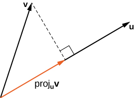
Q11. For given vectors v \bfv v u \bfu u v \bfv v u \bfu u proj u v \proj_\bfu \bfv proj u v u \bfu u v \bfv v y = m x + c y = m x + c y = m x + c
v = [ 2 3 ] \bfv = \begin{bmatrix} 2 \\ 3 \end{bmatrix} v = [ 2 3 ] u = [ 3 2 ] \bfu = \begin{bmatrix} 3 \\ 2 \end{bmatrix} u = [ 3 2 ]
A11.
proj u v = v ⊤ u ∥ u ∥ = 12 13 \proj_\bfu \bfv = \bfv^\top \frac{\bfu}{\|\bfu\|} = \frac{12}{\sqrt{13}} proj u v = v ⊤ ∥ u ∥ u = 13 12
The dotted line is the set of all points x ∈ R 2 \bfx \in \bbR^2 x ∈ R 2 u ⊤ x = u ⊤ v \bfu^\top \bfx = \bfu^\top \bfv u ⊤ x = u ⊤ v
Let x = [ x , y ] \bfx = [x, y] x = [ x , y ] [ 3 , 2 ] [ x y ] = 12 [3, 2] \begin{bmatrix} x \\ y \end{bmatrix} = 12 [ 3 , 2 ] [ x y ] = 12 3 x + 2 y = 12 3x + 2y = 12 3 x + 2 y = 12
Q12. ¶ Convert the following scalar equation into vector form. Your end result should contain m = [ m ; c ] \bfm = [m; c] m = [ m ; c ] y = [ y 1 ; y 2 ; … ; y n ] \bfy = [y_1; y_2; \dots; y_n] y = [ y 1 ; y 2 ; … ; y n ] x = [ x 1 ; x 2 , … , x n ] \bfx = [x_1; x_2, \dots, x_n] x = [ x 1 ; x 2 , … , x n ] 1 n \mathbb{1}_n 1 n
e ( m , c , ( x 1 , y 1 ) , ( x 2 , y 2 ) , … , ( x n , y n ) ) = ( y 1 − ( x 1 m + c ) ) 2 + ( y 2 − ( x 2 m + c ) ) 2 + ⋯ + ( y n − ( x n m + c ) ) 2 e(m, c, (x_1, y_1), (x_2, y_2), \dots, (x_n, y_n)) = (y_1 - (x_1 m + c))^2 + (y_2 - (x_2 m + c))^2 + \dots + (y_n - (x_n m + c))^2 e ( m , c , ( x 1 , y 1 ) , ( x 2 , y 2 ) , … , ( x n , y n )) = ( y 1 − ( x 1 m + c ) ) 2 + ( y 2 − ( x 2 m + c ) ) 2 + ⋯ + ( y n − ( x n m + c ) ) 2 A12.
Recall that the magnitude of a vector ∥ v ∥ = v 1 2 + v 2 2 + ⋯ + v n n \|\bfv\| = \sqrt{v_1^2 + v_2^2 + \dots + v_n^n} ∥ v ∥ = v 1 2 + v 2 2 + ⋯ + v n n
e = [ y 1 − ( m x 1 + c ) y 2 − ( m x 2 + c ) ⋮ y n − ( m x n + c ) ] \bfe = \begin{bmatrix}y_1 - (mx_1 + c)\\ y_2 - (mx_2 + c)\\ \vdots \\ y_n - (mx_n + c)\end{bmatrix} e = ⎣ ⎡ y 1 − ( m x 1 + c ) y 2 − ( m x 2 + c ) ⋮ y n − ( m x n + c ) ⎦ ⎤ The total error is same as minimizing the square of error vector magnitude which is further same as vector product with itself.
e ( m , c , ( x 1 , y 1 ) , ( x 2 , y 2 ) , … , ( x n , y n ) ) = ∥ e ∥ 2 = e ⊤ e e(m, c, (x_1, y_1), (x_2, y_2), \dots, (x_n, y_n)) = \|\bfe\|^2 = \bfe^\top \bfe e ( m , c , ( x 1 , y 1 ) , ( x 2 , y 2 ) , … , ( x n , y n )) = ∥ e ∥ 2 = e ⊤ e Let us define x = [ x 1 ; … ; x n ] \bfx = [x_1; \dots; x_n] x = [ x 1 ; … ; x n ] y = [ y 1 ; … ; y n ] \bfy = [y_1; \dots; y_n] y = [ y 1 ; … ; y n ]
e = y − ( x m + 1 n c ) \bfe = \bfy - (\bfx m + \mathbf{1}_n c) e = y − ( x m + 1 n c ) where 1 n \mathbf{1}_n 1 n m = [ m ; c ] \bfm = [m; c] m = [ m ; c ] x \bfx x 1 n \mathbf{1}_n 1 n X = [ x , 1 n ] ∈ R n × 2 \bfX = [\bfx, \mathbf{1}_n] \in \bbR^{n \times 2} X = [ x , 1 n ] ∈ R n × 2
e = y − X m \bfe = \bfy - \bfX \bfm e = y − Xm Expanding the error magnitude:
∥ e ∥ 2 = ( y − X m ) ⊤ ( y − X m ) = y ⊤ y + m ⊤ X ⊤ X m − 2 y ⊤ X m \|\bfe\|^2 = (\bfy - \bfX \bfm)^\top (\bfy - \bfX \bfm)
\\
= \bfy^\top\bfy + \bfm^\top \bfX^\top \bfX \bfm - 2\bfy^\top \bfX \bfm ∥ e ∥ 2 = ( y − Xm ) ⊤ ( y − Xm ) = y ⊤ y + m ⊤ X ⊤ Xm − 2 y ⊤ Xm Q13: ¶ Convert the following scalar equation into vector form. Your end result should contain m = [ a ; b ; c ] \bfm = [a; b; c] m = [ a ; b ; c ] z = [ z 1 ; z 2 ; … ; z n ] \bfz = [z_1; z_2; \dots; z_n] z = [ z 1 ; z 2 ; … ; z n ] y = [ y 1 ; y 2 ; … ; y n ] \bfy = [y_1; y_2; \dots; y_n] y = [ y 1 ; y 2 ; … ; y n ] x = [ x 1 ; x 2 , … , x n ] \bfx = [x_1; x_2, \dots, x_n] x = [ x 1 ; x 2 , … , x n ] 1 n \mathbb{1}_n 1 n
e ( a , b , c , ( x 1 , y 1 , z 1 ) , ( x 2 , y 2 , z 2 ) , … , ( x n , y n , z n ) ) = ( z 1 − ( x 1 a + y 1 b + c ) ) 2 + ( z 2 − ( x 2 a + y 2 b + c ) ) 2 + ⋯ + ( z n − ( x n a + y n b + c ) ) 2 e(a, b, c, (x_1, y_1, z_1), (x_2, y_2, z_2), \dots, (x_n, y_n, z_n)) = (z_1 - (x_1 a + y_1 b + c))^2 + (z_2 - (x_2 a + y_2 b + c))^2 + \dots + (z_n - (x_n a + y_n b + c))^2 e ( a , b , c , ( x 1 , y 1 , z 1 ) , ( x 2 , y 2 , z 2 ) , … , ( x n , y n , z n )) = ( z 1 − ( x 1 a + y 1 b + c ) ) 2 + ( z 2 − ( x 2 a + y 2 b + c ) ) 2 + ⋯ + ( z n − ( x n a + y n b + c ) ) 2 Q14 ¶ Convert the following vector equation into even more vectorized form.
e ( m 0 , m , ( x 1 , y 1 ) , ( x 2 , y 2 ) , … , ( x n , y n ) ) = ( y 1 − ( x 1 ⊤ m + m 0 ) ) 2 + ( y 2 − ( x 2 ⊤ m + m 0 ) ) 2 + ⋯ + ( y n − ( x n ⊤ m + m 0 ) ) 2 e(m_0, \bfm, (\bfx_1, y_1), (\bfx_2, y_2), \dots, (\bfx_n, y_n)) = (y_1 - (\bfx_1^\top \bfm + m_0))^2 + (y_2 - (\bfx_2^\top \bfm + m_0))^2 + \dots + (y_n - (\bfx_n^\top \bfm + m_0))^2 e ( m 0 , m , ( x 1 , y 1 ) , ( x 2 , y 2 ) , … , ( x n , y n )) = ( y 1 − ( x 1 ⊤ m + m 0 ) ) 2 + ( y 2 − ( x 2 ⊤ m + m 0 ) ) 2 + ⋯ + ( y n − ( x n ⊤ m + m 0 ) ) 2 where m = [ m 1 ; m 2 ; … ; m p ] ∈ R p \bfm = [m_1; m_2; \dots; m_p] \in \bbR^p m = [ m 1 ; m 2 ; … ; m p ] ∈ R p x i = [ x i 1 ; x i 2 ; … ; x i p ] ∈ R p \bfx_i = [x_{i1}; x_{i2}; \dots; x_{ip}] \in \bbR^p x i = [ x i 1 ; x i 2 ; … ; x i p ] ∈ R p i = { 1 , 2 , … n } i = \{1, 2, \dots n\} i = { 1 , 2 , … n }
Your end result should contain q = [ m 0 , m 1 , m 2 , … , m p ] ∈ R p + 1 \bfq = [m_0, m_1, m_2, \dots, m_p] \in \bbR^{p+1} q = [ m 0 , m 1 , m 2 , … , m p ] ∈ R p + 1 y = [ y 1 ; y 2 ; … ; y n ] ∈ R n \bfy = [y_1; y_2; \dots; y_n]\in \bbR^n y = [ y 1 ; y 2 ; … ; y n ] ∈ R n
X = [ x 11 x 12 … x 1 p x 21 x 22 … x 2 p ⋮ ⋮ ⋱ ⋮ x n 1 x n 2 … x n p ] = [ x 1 ⊤ x 2 ⊤ ⋮ x n ⊤ ] ∈ R n × p \begin{align} \bfX =
\begin{bmatrix}x_{11} & x_{12} & \dots & x_{1p}\\
x_{21} & x_{22} & \dots & x_{2p} \\
\vdots & \vdots & \ddots & \vdots\\
x_{n1} & x_{n2} & \dots & x_{np} \end{bmatrix} = \begin{bmatrix}
\bfx_1^\top \\
\bfx_2^\top \\
\vdots\\
\bfx_n^\top \end{bmatrix}
\in \bbR^{n \times p}
\end{align} X = ⎣ ⎡ x 11 x 21 ⋮ x n 1 x 12 x 22 ⋮ x n 2 … … ⋱ … x 1 p x 2 p ⋮ x n p ⎦ ⎤ = ⎣ ⎡ x 1 ⊤ x 2 ⊤ ⋮ x n ⊤ ⎦ ⎤ ∈ R n × p You can define other vectors and matrices as needed, included a vector of all ones like 1 n \mathbb{1}_n 1 n
A15.
Recall that the magnitude of a vector ∥ v ∥ = v 1 2 + v 2 2 + ⋯ + v n n \|\bfv\| = \sqrt{v_1^2 + v_2^2 + \dots + v_n^n} ∥ v ∥ = v 1 2 + v 2 2 + ⋯ + v n n
e = [ y 1 − ( x 1 ⊤ m + m 0 ) y 2 − ( x 2 ⊤ m + m 0 ) ⋮ y n − ( x 2 ⊤ m 2 + m 0 ) ] \bfe = \begin{bmatrix}y_1 - (\bfx_1^\top\bfm + m_0)\\ y_2 - (\bfx_2^\top\bfm + m_0)\\ \vdots \\ y_n - (\bfx_2^\top\bfm_2 + m_0)\end{bmatrix} e = ⎣ ⎡ y 1 − ( x 1 ⊤ m + m 0 ) y 2 − ( x 2 ⊤ m + m 0 ) ⋮ y n − ( x 2 ⊤ m 2 + m 0 ) ⎦ ⎤ The total error is same as minimizing the square of error vector magnitude which is further same as vector product with itself.
e ( m 0 , m , ( x 1 , y 1 ) , ( x 2 , y 2 ) , … , ( x n , y n ) ) = ∥ e ∥ 2 = e ⊤ e e(m_0, \bfm, (\bfx_1, y_1), (\bfx_2, y_2), \dots, (\bfx_n, y_n)) = \|\bfe\|^2 = \bfe^\top \bfe e ( m 0 , m , ( x 1 , y 1 ) , ( x 2 , y 2 ) , … , ( x n , y n )) = ∥ e ∥ 2 = e ⊤ e Let us define X = [ x 1 ⊤ ; … ; x n ⊤ ] \bfX = [\bfx_1^\top; \dots; \bfx_n^\top] X = [ x 1 ⊤ ; … ; x n ⊤ ] y = [ y 1 ; … ; y n ] \bfy = [y_1; \dots; y_n] y = [ y 1 ; … ; y n ]
e = y − ( 1 n m 0 + X m ) \bfe = \bfy - (\mathbf{1}_n m_0 + \bfX \bfm) e = y − ( 1 n m 0 + Xm ) where 1 n \mathbf{1}_n 1 n q = [ m 0 ; m ] \bfq = [m_0; \bfm] q = [ m 0 ; m ] X \bfX X 1 n \mathbf{1}_n 1 n X ˉ = [ 1 n , X ] ∈ R n × ( p + 1 ) \bar{\bfX} = [\mathbf{1}_n, \bfX] \in \bbR^{n \times (p+1)} X ˉ = [ 1 n , X ] ∈ R n × ( p + 1 )
e = y − X ˉ q \bfe = \bfy - \bar{\bfX} \bfq e = y − X ˉ q Expanding the error magnitude:
∥ e ∥ 2 = ( y − X ˉ q ) ⊤ ( y − X ˉ q ) = y ⊤ y + q ⊤ X ˉ ⊤ X ˉ q − 2 y ⊤ X ˉ q \|\bfe\|^2 = (\bfy - \bbfX \bfq)^\top (\bfy - \bbfX \bfq)
\\
= \bfy^\top\bfy + \bfq^\top \bbfX^\top \bbfX \bfq - 2\bfy^\top \bbfX \bfq ∥ e ∥ 2 = ( y − X ˉ q ) ⊤ ( y − X ˉ q ) = y ⊤ y + q ⊤ X ˉ ⊤ X ˉ q − 2 y ⊤ X ˉ q Q16: ¶ Convert the following scalar equation into vector form. Your end result should contain m = [ m ; c ] \bfm = [m; c] m = [ m ; c ] W = Diag ( [ w 1 ; w 2 ; … ; w n ] ) \bfW = \Diag([w_1; w_2; \dots; w_n]) W = Diag ([ w 1 ; w 2 ; … ; w n ]) y = [ y 1 ; y 2 ; … ; y n ] \bfy = [y_1; y_2; \dots; y_n] y = [ y 1 ; y 2 ; … ; y n ] x = [ x 1 ; x 2 , … , x n ] \bfx = [x_1; x_2, \dots, x_n] x = [ x 1 ; x 2 , … , x n ] 1 n \mathbb{1}_n 1 n
e ( m , c , ( x 1 , y 1 , w 1 ) , ( x 2 , y 2 , w 2 ) , … , ( x n , y n , w n ) ) = w 1 2 ( y 1 − ( x 1 m + c ) ) 2 + w 2 2 ( y 2 − ( x 2 m + c ) ) 2 + ⋯ + w n 2 ( y n − ( x n m + c ) ) 2 e(m, c, (x_1, y_1, w_1), (x_2, y_2, w_2), \dots, (x_n, y_n, w_n)) = w_1^2(y_1 - (x_1 m + c))^2 + w_2^2(y_2 - (x_2 m + c))^2 + \dots + w_n^2(y_n - (x_n m + c))^2 e ( m , c , ( x 1 , y 1 , w 1 ) , ( x 2 , y 2 , w 2 ) , … , ( x n , y n , w n )) = w 1 2 ( y 1 − ( x 1 m + c ) ) 2 + w 2 2 ( y 2 − ( x 2 m + c ) ) 2 + ⋯ + w n 2 ( y n − ( x n m + c ) ) 2 The matrix W \bfW W Diag ( [ w 1 ; w 2 ; … ; w n ] ) \Diag([w_1; w_2; \dots; w_n]) Diag ([ w 1 ; w 2 ; … ; w n ]) W \bfW W [ w 1 ; w 2 ; … ; w n ] [w_1; w_2; \dots; w_n] [ w 1 ; w 2 ; … ; w n ]
W = Diag ( [ w 1 ; w 2 ; … ; w n ] ) = [ w 1 0 … 0 0 w 2 … 0 ⋮ ⋮ ⋱ ⋮ 0 0 … w n ] \bfW = \Diag([w_1; w_2; \dots; w_n]) =
\begin{bmatrix}w_1 & 0 & \dots & 0\\
0 & w_2 & \dots & 0\\
\vdots & \vdots & \ddots & \vdots \\
0 & 0 & \dots & w_n\end{bmatrix} W = Diag ([ w 1 ; w 2 ; … ; w n ]) = ⎣ ⎡ w 1 0 ⋮ 0 0 w 2 ⋮ 0 … … ⋱ … 0 0 ⋮ w n ⎦ ⎤ A16:
Recall that the magnitude of a vector ∥ v ∥ = v 1 2 + v 2 2 + ⋯ + v n n \|\bfv\| = \sqrt{v_1^2 + v_2^2 + \dots + v_n^n} ∥ v ∥ = v 1 2 + v 2 2 + ⋯ + v n n
e = [ y 1 − ( m x 1 + c ) y 2 − ( m x 2 + c ) ⋮ y n − ( m x n + c ) ] \bfe = \begin{bmatrix}y_1 - (mx_1 + c)\\ y_2 - (mx_2 + c)\\ \vdots \\ y_n - (mx_n + c)\end{bmatrix} e = ⎣ ⎡ y 1 − ( m x 1 + c ) y 2 − ( m x 2 + c ) ⋮ y n − ( m x n + c ) ⎦ ⎤ and let W = Diag ( [ w 1 ; w 2 ; … ; w n ] ) \bfW = \Diag([w_1; w_2; \dots; w_n]) W = Diag ([ w 1 ; w 2 ; … ; w n ])
Note that
W e = [ w 1 ( y 1 − ( m x 1 + c ) ) w 2 ( y 2 − ( m x 2 + c ) ) ⋮ w 3 ( y n − ( m x n + c ) ) ] \bfW \bfe = \begin{bmatrix}w_1(y_1 - (mx_1 + c))\\ w_2(y_2 - (mx_2 + c))\\ \vdots \\ w_3(y_n - (mx_n + c))\end{bmatrix} We = ⎣ ⎡ w 1 ( y 1 − ( m x 1 + c )) w 2 ( y 2 − ( m x 2 + c )) ⋮ w 3 ( y n − ( m x n + c )) ⎦ ⎤ The total error is same as the square of error vector magnitude
e ( m , c , ( x 1 , y 1 , w 1 ) , ( x 2 , y 2 , w 2 ) , … , ( x n , y n , w n ) ) = w 1 2 ( y 1 − ( x 1 m + c ) ) 2 + w 2 2 ( y 2 − ( x 2 m + c ) ) 2 + ⋯ + w n 2 ( y n − ( x n m + c ) ) 2 = ∥ W e ∥ 2 e(m, c, (x_1, y_1, w_1), (x_2, y_2, w_2), \dots, (x_n, y_n, w_n)) = w_1^2(y_1 - (x_1 m + c))^2 + w_2^2(y_2 - (x_2 m + c))^2 + \dots + w_n^2(y_n - (x_n m + c))^2 = \|\bfW \bfe\|^2 e ( m , c , ( x 1 , y 1 , w 1 ) , ( x 2 , y 2 , w 2 ) , … , ( x n , y n , w n )) = w 1 2 ( y 1 − ( x 1 m + c ) ) 2 + w 2 2 ( y 2 − ( x 2 m + c ) ) 2 + ⋯ + w n 2 ( y n − ( x n m + c ) ) 2 = ∥ We ∥ 2 The square of error vector magnitude is same as dot product with itself,
∥ W e ∥ 2 = ( W e ) ⊤ ( W e ) = e ⊤ W ⊤ W e \|\bfW \bfe\|^2 = (\bfW\bfe)^\top(\bfW\bfe) = \bfe^\top \bfW^\top \bfW \bfe ∥ We ∥ 2 = ( We ) ⊤ ( We ) = e ⊤ W ⊤ We Let us define x = [ x 1 ; … ; x n ] \bfx = [x_1; \dots; x_n] x = [ x 1 ; … ; x n ] y = [ y 1 ; … ; y n ] \bfy = [y_1; \dots; y_n] y = [ y 1 ; … ; y n ]
e = y − ( x m + 1 n c ) \bfe = \bfy - (\bfx m + \mathbf{1}_n c) e = y − ( x m + 1 n c ) where 1 n \mathbf{1}_n 1 n m = [ m ; c ] \bfm = [m; c] m = [ m ; c ] x \bfx x 1 n \mathbf{1}_n 1 n X = [ x , 1 n ] ∈ R n × 2 \bfX = [\bfx, \mathbf{1}_n] \in \bbR^{n \times 2} X = [ x , 1 n ] ∈ R n × 2
e = y − X m \bfe = \bfy - \bfX \bfm e = y − Xm Expanding the error magnitude:
∥ W e ∥ 2 = ( y − X m ) ⊤ W ⊤ W ( y − X m ) = y ⊤ W ⊤ W y + m ⊤ X ⊤ W ⊤ W X m − 2 y ⊤ W ⊤ W X m \|\bfW\bfe\|^2 = (\bfy - \bfX \bfm)^\top \bfW^\top\bfW (\bfy - \bfX \bfm)
\\
= \bfy^\top\bfW^\top\bfW\bfy + \bfm^\top \bfX^\top \bfW^\top\bfW\bfX \bfm - 2\bfy^\top \bfW^\top\bfW\bfX \bfm ∥ We ∥ 2 = ( y − Xm ) ⊤ W ⊤ W ( y − Xm ) = y ⊤ W ⊤ Wy + m ⊤ X ⊤ W ⊤ WXm − 2 y ⊤ W ⊤ WXm Q17: ¶ Using vector derivatives find the minimum of the following vector quadratic function in m \bfm m
arg min m e ( m ) = y ⊤ W ⊤ W y + m ⊤ X ⊤ W ⊤ W X m − 2 y ⊤ W ⊤ W X m \arg~\min_{\bfm} e(\bfm) = \bfy^\top\bfW^\top\bfW\bfy + \bfm^\top \bfX^\top \bfW^\top\bfW\bfX \bfm - 2\bfy^\top \bfW^\top\bfW\bfX \bfm arg m min e ( m ) = y ⊤ W ⊤ Wy + m ⊤ X ⊤ W ⊤ WXm − 2 y ⊤ W ⊤ WXm The dimensions of the each of the variables are given m ∈ R p \bfm \in \bbR^p m ∈ R p y ∈ R n \bfy \in \bbR^n y ∈ R n W ∈ R n × n \bfW \in \bbR^{n \times n} W ∈ R n × n X ∈ R n × p \bfX \in \bbR^{n \times p} X ∈ R n × p
A17:
0 ⊤ = ∂ ∂ m ( y ⊤ W ⊤ W y + m ⊤ X ⊤ W ⊤ W X m − 2 y ⊤ W ⊤ W X m ) = 2 m ∗ ⊤ X ⊤ W ⊤ W X − 2 y ⊤ W ⊤ W X \begin{align}
\mathbf{0}^\top &= \frac{\p }{\p \bfm} (\bfy^\top\bfW^\top\bfW\bfy + \bfm^\top \bfX^\top \bfW^\top\bfW\bfX \bfm - 2\bfy^\top \bfW^\top\bfW\bfX \bfm)\\
&= 2 {\bfm^*}^\top \bfX^\top \bfW^\top \bfW \bfX - 2\bfy^\top \bfW^\top \bfW \bfX
\end{align} 0 ⊤ = ∂ m ∂ ( y ⊤ W ⊤ Wy + m ⊤ X ⊤ W ⊤ WXm − 2 y ⊤ W ⊤ WXm ) = 2 m ∗ ⊤ X ⊤ W ⊤ WX − 2 y ⊤ W ⊤ WX This gives us the solution
m ∗ = ( X ⊤ W ⊤ W X ) − 1 X ⊤ W ⊤ W y \bfm^* = (\bfX^\top \bfW^\top \bfW \bfX)^{-1} \bfX^\top \bfW^\top \bfW \bfy m ∗ = ( X ⊤ W ⊤ WX ) − 1 X ⊤ W ⊤ Wy Q18: ¶ Find the derivative of f ( x ) = ( x − a 1 ) ⊤ A ( x − a 2 ) f(\bfx) = (\bfx - \bfa_1)^\top A (\bfx - \bfa_2) f ( x ) = ( x − a 1 ) ⊤ A ( x − a 2 ) x \bfx x
You can assume A ∈ R n × n A \in \bbR^{n\times n} A ∈ R n × n x , a 1 , a 2 , a 3 , b ∈ R n \bfx, \bfa_1, \bfa_2, \bfa_3, \bfb \in \bbR^n x , a 1 , a 2 , a 3 , b ∈ R n
A18
f ( x ) = ( x − a 1 ) ⊤ A ( x − a 2 ) = x ⊤ A x − a 1 ⊤ A x − x ⊤ A a 2 + a 1 ⊤ A a 2 f(\bfx) = (\bfx - \bfa_1)^\top A (\bfx - \bfa_2)\\
= \bfx^\top A \bfx - \bfa_1^\top A \bfx - \bfx^\top A \bfa_2 + \bfa_1^\top A\bfa_2\\ f ( x ) = ( x − a 1 ) ⊤ A ( x − a 2 ) = x ⊤ A x − a 1 ⊤ A x − x ⊤ A a 2 + a 1 ⊤ A a 2 Note that x ⊤ A a 2 \bfx^\top A \bfa_2 x ⊤ A a 2 x ⊤ A a 2 = a 2 ⊤ A x \bfx^\top A \bfa_2 = \bfa_2^\top A \bfx x ⊤ A a 2 = a 2 ⊤ A x
= x ⊤ A x − ( a 1 + a 2 ) ⊤ A x + a 1 ⊤ A a 2 = \bfx^\top A \bfx - (\bfa_1 + \bfa_2)^\top A \bfx + \bfa_1^\top A\bfa_2 = x ⊤ A x − ( a 1 + a 2 ) ⊤ A x + a 1 ⊤ A a 2 ∂ f ∂ x = 2 x ⊤ A − ( a 1 + a 2 ) ⊤ A = ( 2 x − ( a 1 + a 2 ) ) ⊤ A \frac{\partial f}{\partial \bfx} = 2\bfx^\top A - (\bfa_1 + \bfa_2)^\top A\\
= (2\bfx - (\bfa_1 + \bfa_2))^\top A ∂ x ∂ f = 2 x ⊤ A − ( a 1 + a 2 ) ⊤ A = ( 2 x − ( a 1 + a 2 ) ) ⊤ A Q19: ¶ Find the quadratic approximation of the following function near the point x 0 \bfx_0 x 0
f ( x ) = ( ( x − a 1 ) ⊤ A ( x − a 2 ) ) ( ( x − a 3 ) ⊤ b ) f(\bfx) = \left((\bfx - \bfa_1)^\top A (\bfx - \bfa_2)\right) \left((\bfx - \bfa_3)^\top \bfb\right) f ( x ) = ( ( x − a 1 ) ⊤ A ( x − a 2 ) ) ( ( x − a 3 ) ⊤ b ) You can assume A ∈ R n × n A \in \bbR^{n\times n} A ∈ R n × n x , a 1 , a 2 , a 3 , b ∈ R n \bfx, \bfa_1, \bfa_2, \bfa_3, \bfb \in \bbR^n x , a 1 , a 2 , a 3 , b ∈ R n
A19:
[ ∇ x f ( x ) ] ⊤ = ( ( x − a 1 ) ⊤ A ( x − a 2 ) ) b ⊤ + ( ( x − a 3 ) ⊤ b ) ( ( 2 x − ( a 1 + a 2 ) ) ⊤ A ) [\nabla_\bfx f(\bfx)]^\top = \left((\bfx - \bfa_1)^\top A (\bfx - \bfa_2)\right) \bfb^\top+ ((\bfx - \bfa_3)^\top \bfb)\left((2\bfx - (\bfa_1 + \bfa_2))^\top A\right) [ ∇ x f ( x ) ] ⊤ = ( ( x − a 1 ) ⊤ A ( x − a 2 ) ) b ⊤ + (( x − a 3 ) ⊤ b ) ( ( 2 x − ( a 1 + a 2 ) ) ⊤ A ) ∇ x f ( x ) = ( ( x − a 1 ) ⊤ A ( x − a 2 ) ) b + ( ( x − a 3 ) ⊤ b ) ( A ( 2 x − ( a 1 + a 2 ) ) ) \nabla_\bfx f(\bfx) = \left((\bfx - \bfa_1)^\top A (\bfx - \bfa_2)\right) \bfb + ((\bfx - \bfa_3)^\top \bfb)\left(A (2\bfx - (\bfa_1 + \bfa_2))\right) ∇ x f ( x ) = ( ( x − a 1 ) ⊤ A ( x − a 2 ) ) b + (( x − a 3 ) ⊤ b ) ( A ( 2 x − ( a 1 + a 2 )) ) ∇ x f ( x 0 ) = ( ( x 0 − a 1 ) ⊤ A ( x 0 − a 2 ) ) b + ( ( x 0 − a 3 ) ⊤ b ) ( A ( 2 x 0 − ( a 1 + a 2 ) ) ) \nabla_\bfx f(\bfx_0) = \left((\bfx_0 - \bfa_1)^\top A (\bfx_0 - \bfa_2)\right) \bfb + ((\bfx_0 - \bfa_3)^\top \bfb)\left(A (2\bfx_0 - (\bfa_1 + \bfa_2))\right) ∇ x f ( x 0 ) = ( ( x 0 − a 1 ) ⊤ A ( x 0 − a 2 ) ) b + (( x 0 − a 3 ) ⊤ b ) ( A ( 2 x 0 − ( a 1 + a 2 )) ) H f ( x ) = ∇ x 2 f ( x ) = b ( 2 x − ( a 1 + a 2 ) ) ⊤ A + ( A ( 2 x − ( a 1 + a 2 ) ) ) b ⊤ + ( ( x − a 3 ) ⊤ b ) ( 2 A ) H f(\bfx) = \nabla^2_\bfx f(\bfx) = \bfb (2\bfx - (\bfa_1 + \bfa_2))^\top A
+ \left(A (2\bfx - (\bfa_1 + \bfa_2))\right)\bfb^\top
+ \left((\bfx - \bfa_3)^\top \bfb\right)(2A) H f ( x ) = ∇ x 2 f ( x ) = b ( 2 x − ( a 1 + a 2 ) ) ⊤ A + ( A ( 2 x − ( a 1 + a 2 )) ) b ⊤ + ( ( x − a 3 ) ⊤ b ) ( 2 A ) H f ( x 0 ) = ∇ x 2 f ( x 0 ) = b ( 2 x 0 − ( a 1 + a 2 ) ) ⊤ A + ( A ( 2 x 0 − ( a 1 + a 2 ) ) ) b ⊤ + ( ( x 0 − a 3 ) ⊤ b ) ( 2 A ) H f(\bfx_0) = \nabla^2_\bfx f(\bfx_0) = \bfb (2\bfx_0 - (\bfa_1 + \bfa_2))^\top A
+ \left(A (2\bfx_0 - (\bfa_1 + \bfa_2))\right)\bfb^\top
+ \left((\bfx_0 - \bfa_3)^\top \bfb\right)(2A) H f ( x 0 ) = ∇ x 2 f ( x 0 ) = b ( 2 x 0 − ( a 1 + a 2 ) ) ⊤ A + ( A ( 2 x 0 − ( a 1 + a 2 )) ) b ⊤ + ( ( x 0 − a 3 ) ⊤ b ) ( 2 A ) The quadratic approximation by Taylor series is:
f ( x ) = f ( x 0 ) + [ ∇ x f ( x 0 ) ] ⊤ ( x − x 0 ) + ( x − x 0 ) ⊤ H f ( x 0 ) ( x − x 0 ) f(\bfx) = f(\bfx_0) + [\nabla_\bfx f(\bfx_0)]^\top (\bfx - \bfx_0) + (\bfx - \bfx_0)^\top H f(\bfx_0) (\bfx - \bfx_0) f ( x ) = f ( x 0 ) + [ ∇ x f ( x 0 ) ] ⊤ ( x − x 0 ) + ( x − x 0 ) ⊤ H f ( x 0 ) ( x − x 0 ) Q20 ¶ Show that for c , x ∈ R n \bfc, \bfx \in \bbR^n c , x ∈ R n
∂ ∂ x c ⊤ x = c ⊤ \begin{align}
\frac{\p }{ \p \bfx} \bfc^\top \bfx = \bfc^\top\\
\end{align} ∂ x ∂ c ⊤ x = c ⊤ A20:
Let c = [ c 1 , c 2 , … , c n ] \bfc = [c_1, c_2, \dots, c_n] c = [ c 1 , c 2 , … , c n ] x = [ x 1 , x 2 , … x n ] \bfx = [x_1, x_2, \dots x_n] x = [ x 1 , x 2 , … x n ]
Let f ( x ) = c ⊤ x = c 1 x 1 + c 2 x 2 + … c n x n f(\bfx) = \bfc^\top \bfx = c_1 x_1 + c_2 x_2 + \dots c_n x_n f ( x ) = c ⊤ x = c 1 x 1 + c 2 x 2 + … c n x n
∂ f ∂ x 1 = c 1 ∂ f ∂ x 2 = c 2 ⋮ ∂ f ∂ x n = c n \frac{\p f}{\p x_1} = c_1\\
\frac{\p f}{\p x_2} = c_2\\
\vdots\\
\frac{\p f}{\p x_n} = c_n\\ ∂ x 1 ∂ f = c 1 ∂ x 2 ∂ f = c 2 ⋮ ∂ x n ∂ f = c n By Jacobian convention, we arrange the partial derivatives in a row vector:
∂ ∂ x c ⊤ x = [ ∂ f ∂ x 1 ∂ f ∂ x 2 … ∂ f ∂ x n ] = [ c 1 c 2 … c n ] = c ⊤ \begin{align}
\frac{\p }{ \p \bfx} \bfc^\top \bfx =
\begin{bmatrix} \frac{\p f}{\p x_1} & \frac{\p f}{\p x_2} & \dots & \frac{\p f}{\p x_n}\end{bmatrix}
\\
= \begin{bmatrix} c_1 & c_2 & \dots & c_n\end{bmatrix} = \bfc^\top \\
\end{align} ∂ x ∂ c ⊤ x = [ ∂ x 1 ∂ f ∂ x 2 ∂ f … ∂ x n ∂ f ] = [ c 1 c 2 … c n ] = c ⊤ Q21: ¶ Show that for A ∈ R n × n \bfA \in \bbR^{n \times n} A ∈ R n × n x ∈ R n \bfx \in \bbR^n x ∈ R n
∂ ∂ x A x = A \begin{align}
\frac{\p }{ \p \bfx} \bfA \bfx = \bfA\\
\end{align} ∂ x ∂ Ax = A A21:
Let x = [ x 1 ; x 2 ; … x n ] \bfx = [x_1; x_2; \dots x_n] x = [ x 1 ; x 2 ; … x n ]
Let A = [ a 11 a 12 … a 1 n a 21 a 22 … a 2 n ⋮ ⋮ ⋱ ⋮ a n 1 a n 2 … a n n ] = [ a 1 ⊤ a 2 ⊤ ⋮ a n ⊤ ] \bfA = \begin{bmatrix} a_{11} & a_{12} & \dots & a_{1n} \\
a_{21} & a_{22} & \dots & a_{2n} \\
\vdots & \vdots & \ddots & \vdots \\
a_{n1} & a_{n2} & \dots & a_{nn} \end{bmatrix}
= \begin{bmatrix} \bfa_1^\top \\ \bfa_2^\top \\ \vdots \\ \bfa_n^\top \end{bmatrix} A = ⎣ ⎡ a 11 a 21 ⋮ a n 1 a 12 a 22 ⋮ a n 2 … … ⋱ … a 1 n a 2 n ⋮ a nn ⎦ ⎤ = ⎣ ⎡ a 1 ⊤ a 2 ⊤ ⋮ a n ⊤ ⎦ ⎤ a i ⊤ ∈ R 1 × n \bfa_i^\top \in \bbR^{1 \times n} a i ⊤ ∈ R 1 × n A \bfA A
Then
A x = [ a 1 ⊤ a 2 ⊤ ⋮ a n ⊤ ] x = [ a 1 ⊤ x a 2 ⊤ x ⋮ a n ⊤ x ] \bfA \bfx = \begin{bmatrix} \bfa_1^\top \\ \bfa_2^\top \\ \vdots \\ \bfa_n^\top \end{bmatrix}\bfx
= \begin{bmatrix} \bfa_1^\top \bfx \\ \bfa_2^\top \bfx \\ \vdots \\ \bfa_n^\top\bfx \end{bmatrix} Ax = ⎣ ⎡ a 1 ⊤ a 2 ⊤ ⋮ a n ⊤ ⎦ ⎤ x = ⎣ ⎡ a 1 ⊤ x a 2 ⊤ x ⋮ a n ⊤ x ⎦ ⎤ Let
$$\bff(\bfx) =
[ f 1 ( x ) f 2 ( x ) ⋮ f n ( x ) ] \begin{bmatrix} f_1(\bfx) \\ f_2(\bfx) \\ \vdots\\ f_n(\bfx) \end{bmatrix} ⎣ ⎡ f 1 ( x ) f 2 ( x ) ⋮ f n ( x ) ⎦ ⎤ = \bfA \bfx = \begin{bmatrix} \bfa_1^\top \bfx \ \bfa_2^\top \bfx \ \vdots \ \bfa_n^\top\bfx \end{bmatrix}$$
By Jacobian convention we arrange the partial derivatives of each function component column-wise
∂ f ( x ) ∂ x = [ ∂ f 1 ( x ) ∂ x ∂ f 2 ( x ) ∂ x ⋮ ∂ f n ( x ) ∂ x ] = [ ∂ a 1 ⊤ x ∂ x ∂ a 2 ⊤ x ∂ x ⋮ ∂ a 2 ⊤ x ∂ x ] = [ a 1 ⊤ a 2 ⊤ ⋮ a n ⊤ ] = A \frac{\p \bff(\bfx)}{\p \bfx} =
\begin{bmatrix} \frac{\p f_1(\bfx)}{\p \bfx} \\
\frac{\p f_2(\bfx)}{\p \bfx} \\
\vdots \\
\frac{\p f_n(\bfx)}{\p \bfx} \end{bmatrix}
= \begin{bmatrix} \frac{\p \bfa_1^\top \bfx}{\p \bfx} \\
\frac{\p \bfa_2^\top \bfx}{\p \bfx} \\
\vdots \\
\frac{\p \bfa_2^\top \bfx}{\p \bfx} \end{bmatrix}
= \begin{bmatrix} \bfa_1^\top \\ \bfa_2^\top \\ \vdots \\ \bfa_n^\top \end{bmatrix}
= \bfA ∂ x ∂ f ( x ) = ⎣ ⎡ ∂ x ∂ f 1 ( x ) ∂ x ∂ f 2 ( x ) ⋮ ∂ x ∂ f n ( x ) ⎦ ⎤ = ⎣ ⎡ ∂ x ∂ a 1 ⊤ x ∂ x ∂ a 2 ⊤ x ⋮ ∂ x ∂ a 2 ⊤ x ⎦ ⎤ = ⎣ ⎡ a 1 ⊤ a 2 ⊤ ⋮ a n ⊤ ⎦ ⎤ = A Q22: ¶ Use vector-derivative chain rule:
∂ f ( g ( x ) ) ∂ x = ∂ f ∂ g ∂ g ∂ x \frac{\p \bff(\bfg(\bfx)) }{\p \bfx} = \frac{\p \bff}{\p \bfg}\frac{\p \bfg}{\p \bfx} ∂ x ∂ f ( g ( x )) = ∂ g ∂ f ∂ x ∂ g ,
for any function g : R n ↦ R m \bfg : \bbR^n \mapsto \bbR^m g : R n ↦ R m f : R m ↦ R o \bff : \bbR^m \mapsto \bbR^o f : R m ↦ R o
Show that for x ∈ R n \bfx \in \bbR^n x ∈ R n A ∈ R n × n \bfA \in \bbR^{n \times n} A ∈ R n × n
∂ ∂ x x ⊤ A x = x ⊤ ( A ⊤ + A ) \begin{align}
\frac{\p }{ \p \bfx} \bfx^\top \bfA \bfx = \bfx^\top (\bfA^\top + \bfA)\\
\end{align} ∂ x ∂ x ⊤ Ax = x ⊤ ( A ⊤ + A ) A22:
For product of any two vectors
∂ ∂ x x ⊤ y = y ⊤ \begin{align}
\frac{\p }{\p \bfx} \bfx^\top \bfy = \bfy^\top
\end{align} ∂ x ∂ x ⊤ y = y ⊤ If y \bfy y x \bfx x
∂ ∂ x x ⊤ y = y ⊤ + ( ∂ ∂ y x ⊤ y ) ( ∂ y ∂ x ) = y ⊤ + x ⊤ ( ∂ y ∂ x ) \begin{align}
\frac{\p }{\p \bfx} \bfx^\top \bfy &= \bfy^\top +
\left(\frac{\p }{\p \bfy} \bfx^\top \bfy \right) \left(\frac{\p \bfy }{\p \bfx} \right)\\
&= \bfy^\top + \bfx^\top \left(\frac{\p \bfy }{\p \bfx}\right)
\end{align} ∂ x ∂ x ⊤ y = y ⊤ + ( ∂ y ∂ x ⊤ y ) ( ∂ x ∂ y ) = y ⊤ + x ⊤ ( ∂ x ∂ y ) If y = A x \bfy = \bfA \bfx y = Ax
∂ y ∂ x = ∂ ∂ x A x = A \frac{\p \bfy}{\p \bfx} = \frac{\p }{\p \bfx} \bfA \bfx = \bfA ∂ x ∂ y = ∂ x ∂ Ax = A and
∂ ∂ x x ⊤ A x = y ⊤ + x ⊤ ( ∂ y ∂ x ) = x ⊤ A ⊤ + x ⊤ A = x ⊤ ( A ⊤ + A ) \frac{\p }{\p \bfx} \bfx^\top \bfA \bfx =
\bfy^\top + \bfx^\top \left(\frac{\p \bfy }{\p \bfx}\right)
= \bfx^\top \bfA^\top + \bfx^\top \bfA
= \bfx^\top (\bfA^\top + \bfA) ∂ x ∂ x ⊤ Ax = y ⊤ + x ⊤ ( ∂ x ∂ y ) = x ⊤ A ⊤ + x ⊤ A = x ⊤ ( A ⊤ + A ) Q23: ¶ You are given 2D points and corresponding labels as a training dataset { ( x 1 , y 1 , l 1 ) , ( x 2 , y 2 , l 2 ) , … , ( x n , y n , l n ) } \{ (x_1, y_1, l_1), (x_2, y_2, l_2), \dots, (x_n, y_n, l_n) \} {( x 1 , y 1 , l 1 ) , ( x 2 , y 2 , l 2 ) , … , ( x n , y n , l n )} x i ∈ R x_i \in \bbR x i ∈ R y i ∈ R y_i \in \bbR y i ∈ R l i ∈ { − 1 , 1 } l_i \in \{-1, 1\} l i ∈ { − 1 , 1 } l ^ i = sign ( y i − ( m x i + c ) ) \hat{l}_i = \sign(y_i - (m x_i + c)) l ^ i = sign ( y i − ( m x i + c )) m = [ m ; c ] \bfm = [m; c] m = [ m ; c ]
A23
e ( y i , x i ; m , c ) = { 0 if sign ( y i − ( m x i + c ) ) = l i ∣ y i − ( m x i + c ) ∣ if sign ( y i − ( m x i + c ) ) ≠ l i e(y_i, x_i; m,c) = \begin{cases}
0 &\text{ if }\sign(y_i - (m x_i + c)) = l_i\\
|y_i - (m x_i + c)| &\text{ if } \sign(y_i - (m x_i + c)) \ne l_i
\end{cases} e ( y i , x i ; m , c ) = { 0 ∣ y i − ( m x i + c ) ∣ if sign ( y i − ( m x i + c )) = l i if sign ( y i − ( m x i + c )) = l i m = [ m c ] \bfm = \begin{bmatrix}m \\ c\end{bmatrix} m = [ m c ] e ( y i , x i ; m ) = { 0 if sign ( y i − [ x i 1 ] m ) = l i ∣ y i − [ x i 1 ] m ∣ if sign ( y i − [ x i 1 ] m ) ≠ l i e(y_i, x_i;\bfm) = \begin{cases}
0 &\text{ if } \sign( y_i - \begin{bmatrix} x_i& 1\end{bmatrix}\bfm) = l_i\\
|y_i - \begin{bmatrix} x_i& 1\end{bmatrix}\bfm| &\text{ if } \sign( y_i - \begin{bmatrix} x_i& 1\end{bmatrix}\bfm) \ne l_i
\end{cases} e ( y i , x i ; m ) = { 0 ∣ y i − [ x i 1 ] m ∣ if sign ( y i − [ x i 1 ] m ) = l i if sign ( y i − [ x i 1 ] m ) = l i If l i ∈ { − 1 , 1 } l_i \in \{-1, 1\} l i ∈ { − 1 , 1 } sign ( y i − [ x i 1 ] m ) = l i \sign( y_i - \begin{bmatrix} x_i& 1\end{bmatrix}\bfm) = l_i sign ( y i − [ x i 1 ] m ) = l i l i ( y i − [ x i 1 ] m ) > 0 l_i( y_i - \begin{bmatrix} x_i& 1\end{bmatrix}\bfm) > 0 l i ( y i − [ x i 1 ] m ) > 0
e ( y i , x i ; m ) = { 0 if l i ( y i − [ x i 1 ] m ) > 0 ∣ l i ( y i − [ x i 1 ] m ) ∣ if l i ( y i − [ x i 1 ] m ) < 0 e(y_i, x_i;\bfm) = \begin{cases}
0 &\text{ if } l_i( y_i - \begin{bmatrix} x_i& 1\end{bmatrix}\bfm) > 0\\
|l_i( y_i - \begin{bmatrix} x_i& 1\end{bmatrix}\bfm)| &\text{ if } l_i( y_i - \begin{bmatrix} x_i& 1\end{bmatrix}\bfm) < 0
\end{cases} e ( y i , x i ; m ) = { 0 ∣ l i ( y i − [ x i 1 ] m ) ∣ if l i ( y i − [ x i 1 ] m ) > 0 if l i ( y i − [ x i 1 ] m ) < 0 Also when z < 0 z < 0 z < 0 ∣ z ∣ = − z |z| = -z ∣ z ∣ = − z
e ( y i , x i ; m ) = { 0 if l i ( y i − [ x i 1 ] m ) > 0 − l i ( y i − [ x i 1 ] m ) if l i ( y i − [ x i 1 ] m ) < 0 e(y_i, x_i;\bfm) = \begin{cases}
0 &\text{ if } l_i( y_i - \begin{bmatrix} x_i& 1\end{bmatrix}\bfm) > 0\\
-l_i( y_i - \begin{bmatrix} x_i& 1\end{bmatrix}\bfm) &\text{ if } l_i( y_i - \begin{bmatrix} x_i& 1\end{bmatrix}\bfm) < 0
\end{cases} e ( y i , x i ; m ) = { 0 − l i ( y i − [ x i 1 ] m ) if l i ( y i − [ x i 1 ] m ) > 0 if l i ( y i − [ x i 1 ] m ) < 0 e ( y i , x i ; m ) = max { 0 , − l i ( y i − [ x i 1 ] m ) } e(y_i, x_i;\bfm) = \max\{0, - l_i (y_i - \begin{bmatrix} x_i& 1\end{bmatrix}\bfm)\} e ( y i , x i ; m ) = max { 0 , − l i ( y i − [ x i 1 ] m )} ∇ m e ( y i , x i ; m ) = max { 0 , l i ( [ x i 1 ] ) } \nabla_\bfm e(y_i, x_i;\bfm) = \max\{0, l_i(\begin{bmatrix} x_i& 1\end{bmatrix})\} ∇ m e ( y i , x i ; m ) = max { 0 , l i ( [ x i 1 ] )} For the entire dataset, we have y = [ y 1 ; … ; y n ] \bfy = [y_1; \dots; y_n] y = [ y 1 ; … ; y n ] x = [ x 1 ; … ; x n ] \bfx = [x_1; \dots; x_n] x = [ x 1 ; … ; x n ] ℓ = [ l 1 ; … ; l n ] \ell = [l_1; \dots; l_n] ℓ = [ l 1 ; … ; l n ]
e ( x , y ; m ) = 1 n 1 n ⊤ max { 0 , − ℓ ⊙ ( y − [ x 1 n ] m ) } , e(\bfx, \bfy; \bfm) = \frac{1}{n}{\bfone_n^\top}\max\{0, - \ell \odot (\bfy - \begin{bmatrix}\bfx & \bfone_n\end{bmatrix}\bfm )\}, e ( x , y ; m ) = n 1 1 n ⊤ max { 0 , − ℓ ⊙ ( y − [ x 1 n ] m )} , where ⊙ \odot ⊙ 1 n \bfone_n 1 n
and the average gradient is:
∇ m ⊤ e ( x , y ; m ) = 1 n 1 n ⊤ max { 0 , ℓ ⊙ ( [ x 1 n ] ) } \nabla_\bfm^\top e(\bfx, \bfy; \bfm) = \frac{1}{n}{\bfone_n^\top}\max\{0, \ell \odot ( \begin{bmatrix}\bfx & \bfone_n\end{bmatrix} )\} ∇ m ⊤ e ( x , y ; m ) = n 1 1 n ⊤ max { 0 , ℓ ⊙ ( [ x 1 n ] )} Q24 ¶ You are given p-D points x i ∈ R p \bfx_i \in \bbR^p x i ∈ R p { ( x 1 , l 1 ) , ( x 2 , l 2 ) , … , ( x n , l n ) } \{ (\bfx_1, l_1), (\bfx_2, l_2), \dots, (\bfx_n, l_n) \} {( x 1 , l 1 ) , ( x 2 , l 2 ) , … , ( x n , l n )} x i ∈ R p \bfx_i \in \bbR^p x i ∈ R p l i ∈ { − 1 , 1 } l_i \in \{-1, 1\} l i ∈ { − 1 , 1 } l ^ i = sign ( x i ⊤ m + m 0 ) ) \hat{l}_i = \sign(\bfx_i^\top \bfm + m_0)) l ^ i = sign ( x i ⊤ m + m 0 )) q = [ m 0 ; m ] \bfq = [m_0; \bfm] q = [ m 0 ; m ]
A24:
e ( m 0 , m ; x i ) = { 0 if sign ( x i ⊤ m + m 0 ) = l i ∣ x i ⊤ m + m 0 ∣ if sign ( x i ⊤ m + m 0 ) ≠ l i e(m_0, \bfm; \bfx_i) = \begin{cases}
0 &\text{ if }\sign(\bfx_i^\top \bfm + m_0) = l_i\\
|\bfx_i^\top \bfm + m_0| &\text{ if } \sign(\bfx_i^\top \bfm + m_0) \ne l_i
\end{cases} e ( m 0 , m ; x i ) = { 0 ∣ x i ⊤ m + m 0 ∣ if sign ( x i ⊤ m + m 0 ) = l i if sign ( x i ⊤ m + m 0 ) = l i e ( y i , x i ; m , c ) = { 0 if sign ( x i ⊤ m + m 0 ) = l i ∣ x i ⊤ m + m 0 ∣ if sign ( x i ⊤ m + m 0 ) ≠ l i e(y_i, x_i; m, c) = \begin{cases}
0 &\text{ if } \sign(\bfx_i^\top \bfm + m_0) = l_i\\
|\bfx_i^\top \bfm + m_0| &\text{ if } \sign(\bfx_i^\top \bfm + m_0) \ne l_i
\end{cases} e ( y i , x i ; m , c ) = { 0 ∣ x i ⊤ m + m 0 ∣ if sign ( x i ⊤ m + m 0 ) = l i if sign ( x i ⊤ m + m 0 ) = l i q = [ m 0 m ] \bfq = \begin{bmatrix}m_0 \\ \bfm\end{bmatrix} q = [ m 0 m ] e ( m 0 , m ; x i ) = { 0 if [ 1 x i ⊤ ] q = l i ∣ [ 1 x i ⊤ ] q ∣ if [ 1 x i ⊤ ] q ≠ l i e(m_0, \bfm;\bfx_i) = \begin{cases}
0 &\text{ if } \begin{bmatrix} 1 & \bfx_i^\top\end{bmatrix}\bfq = l_i\\
|\begin{bmatrix} 1 & \bfx_i^\top\end{bmatrix}\bfq| &\text{ if } \begin{bmatrix} 1 & \bfx_i^\top\end{bmatrix}\bfq \ne l_i
\end{cases} e ( m 0 , m ; x i ) = { 0 ∣ [ 1 x i ⊤ ] q ∣ if [ 1 x i ⊤ ] q = l i if [ 1 x i ⊤ ] q = l i If l i ∈ { − 1 , 1 } l_i \in \{-1, 1\} l i ∈ { − 1 , 1 }
e ( m 0 , m ; x i ) = max { 0 , − l i ( [ 1 x i ⊤ ] q ) } e(m_0, \bfm;\bfx_i) = \max\{0, - l_i (\begin{bmatrix} 1 & \bfx_i^\top\end{bmatrix}\bfq)\} e ( m 0 , m ; x i ) = max { 0 , − l i ( [ 1 x i ⊤ ] q )} ∇ m e ( m 0 , m ; x i ) = max { 0 , − l i ( [ 1 x i ⊤ ] ) } \nabla_\bfm e(m_0, \bfm;\bfx_i) = \max\{0, - l_i (\begin{bmatrix} 1 & \bfx_i^\top\end{bmatrix})\} ∇ m e ( m 0 , m ; x i ) = max { 0 , − l i ( [ 1 x i ⊤ ] )} For the entire dataset, we have X = [ x 1 ⊤ ; … ; x n ⊤ ] \bfX = [\bfx_1^\top; \dots; \bfx_n^\top] X = [ x 1 ⊤ ; … ; x n ⊤ ] l = [ l 1 ; … ; l n ] \bfl = [l_1; \dots; l_n] l = [ l 1 ; … ; l n ]
e ( m ; X , l ) = 1 n 1 n ⊤ max { 0 , − l ⊙ ( [ 1 n X ] q ) } e(\bfm; \bfX, \bfl) = \frac{1}{n}{\bfone_n^\top}\max\{0, - \bfl \odot ( \begin{bmatrix}\bfone_n & \bfX \end{bmatrix}\bfq )\} e ( m ; X , l ) = n 1 1 n ⊤ max { 0 , − l ⊙ ( [ 1 n X ] q )} and the average gradient is:
∇ m ⊤ e ( m ; X , l ) = 1 n 1 n ⊤ max { 0 , l ⊙ ( [ 1 n X ] ) } \nabla_\bfm^\top e(\bfm; \bfX, \bfl) = \frac{1}{n}{\bfone_n^\top}\max\{0, \bfl \odot ( \begin{bmatrix} \bfone_n & \bfX \end{bmatrix} )\} ∇ m ⊤ e ( m ; X , l ) = n 1 1 n ⊤ max { 0 , l ⊙ ( [ 1 n X ] )}