Visualizing eigen vectors - Neural Networks

Helper functions¶

import numpy as np
def random_symmetric_matrix(n):
    A = np.random.rand(n, n)
    return A + A.T

def random_positive_definite_matrix(n):
    A = np.random.rand(n, n)
    return A.T @ A

import matplotlib.pyplot as plt
def plot_contour(ax, func):
    x, y = np.mgrid[-2:2:21j,
                    -2:2:21j]
    bfx = np.concatenate([x[..., None], y[..., None]], axis=-1)
    f = func(bfx)
    ctr = ax.contour(x, y, f, 20, cmap='Blues_r')
    plt.clabel(ctr, ctr.levels, inline=True, fontsize=6)
    ax.set_xlabel('$x$')
    ax.set_ylabel('$y$')
    return ax


def draw_arrows(ax, xs):
    ax.arrow(0, 0, xs[0, 0], xs[0, 1], color='r', head_width=0.05)
    ax.arrow(0, 0, xs[1, 0], xs[1, 1], color='y', head_width=0.05)
    ax.axis('equal')
    return ax

def f(x, A=np.array([[2, -1], [-1, 3]])):
    # x is m x m x n tensor
    x_row_vec = x[..., None, :] # m x m x 1 x n
    x_col_vec = x[..., :, None] # m x m x n x 1
    res = x_row_vec @ A @ x_col_vec # m x m x 1 x 1
    return res[..., 0, 0] # m x m

fig, ax = plt.subplots()
plot_contour(ax, f)
ax

<Axes: xlabel='$x$', ylabel='$y$'>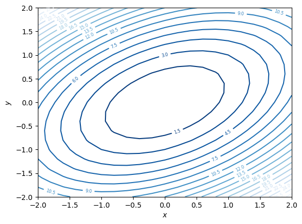

Eigeven value decomposition¶

Recall that eigen values $\lambda \in \bbR$ and eigen vectors $\bfv \in \bbR^n$ are the solutions to the equation,

A \bfv = \lambda \bfv

(1)

There are $n$ such solutions let $\lambda_i$ $\bfv_i$ for $i \in \{ 1, \dots, n\}$ be such solutions.

\begin{align} A\bfv_1 &= \lambda_1 \bfv_1 \\ A\bfv_2 &= \lambda_2 \bfv_2 \\ \vdots &\\ A\bfv_n &= \lambda_n \bfv_n \end{align}

(2)

You can arrange these equations in a matrix $$

\begin{bmatrix} A\bfv_1 & A\bfv_2 & \dots & A\bfv_n \end{bmatrix}

(3)

=

\begin{bmatrix} \lambda_1\bfv_1 & \lambda_2\bfv_2 & \dots & \lambda_n\bfv_n \end{bmatrix}

(4)

$$

You can take $A$ common from the left hand side. On the right hand side, you will have to construct a diagonal matrix of $\lambda_i$ for factorizing eigen vectors and eigen values.

A \underbrace{ \begin{bmatrix} \bfv_1 & \bfv_2 & \dots & \bfv_n \end{bmatrix}}_{V} = \underbrace{ \begin{bmatrix} \bfv_1 & \bfv_2 & \dots & \bfv_n \end{bmatrix}}_{V} \underbrace{ \begin{bmatrix} \lambda_1 & 0 & \dots & 0\\ 0 & \lambda_2 & \dots & 0\\ \vdots & \vdots & \ddots & \vdots \\ 0 & 0 & \dots & \lambda_n \end{bmatrix}}_{\Lambda}

(5)

Homework (VisEigenVectors): Problem 1¶

(10 marks)

Prove that

\begin{bmatrix} \lambda_1\bfv_1 & \lambda_2\bfv_2 & \dots & \lambda_n\bfv_n \end{bmatrix} = \begin{bmatrix} \bfv_1 & \bfv_2 & \dots & \bfv_n \end{bmatrix} \begin{bmatrix} \lambda_1 & 0 & \dots & 0\\ 0 & \lambda_2 & \dots & 0\\ \vdots & \vdots & \ddots & \vdots \\ 0 & 0 & \dots & \lambda_n \end{bmatrix}

(6)

Verify that the above matrix multiplication gives the same results.

A V = V\Lambda

(7)

$V$ is a matrix of eigen vectors arranged as columns. And $\Lambda$ is a diagonal matrix of eigen values.

If the matrix $V$ is invertible, then we can right multiply $V^{-1}$ to both sides,

A = V \Lambda V^{-1}

(8)

We have found a way to factorize (or decompose) a square matrix $A$ . This particular decomposition is called Eigen value decomposition. When such a decomposition exists, the matrix $A$ is called diagonalizable. A generalized form of such decomposition also exists, which is called generalized eigen value decomposition, where the middle matrix is a block diagonal matrix, not diagonal matrix.

Theorem: Symmeteric matrices have orthonormal Eigen vectors¶

When a square matrix $A \in \bbR^{n \times n}$ is real and symmetric, then its Eigen value decomposition exists, $A$ is diagonalizable, and the eigen matrix $V$ is an orthogonal matrix.

If the matrix $A$ is symmetric,

A = V\Lambda V^\top

(9)

where $V^{-1} = V^\top$ .

Proof:¶

Proof will take too much time out of the class. Interested readers are encouraged to read about Gram-Schmidt orthogonalization, Schur’s lemma and Spectral theorem.

Definition (Orthonormal)¶

A matrix $V \in \bbR^{n \times n}$ is called orthonormal or orthogonal if $V^\top V = I_n$ equivalently, $V^{-1} = V^\top$ .

Example¶

Consider the quadratic form of a symmetric matrix $A \in \bbR^{n \times n}$ ,

f(\bfx) = \bfx^\top A \bfx

(10)

Because the matrix $A$ is symmetric, we can write

f(\bfx) = \bfx^\top V\Lambda V^\top \bfx = (V\bfx)^\top \Lambda (V\bfx)

(11)

for eigen value decomposition of $A = V\Lambda V^\top$

A = np.array([[2, -1],
             [-1, 3]])
A

array([[ 2, -1],
       [-1,  3]])

np.linalg.eigh finds Eigen values of a Hermitian matrix.

lambdas, V = np.linalg.eigh(A)

array([[-0.85065081, -0.52573111],
       [-0.52573111,  0.85065081]])

Definition (Conjugate transpose)¶

Conjugate transpose of a complex square matrix $A \in \bbC^{n \times n}$ is defined as

A^H = Re(A)^\top - \iota Im(A)^\top,

(12)

where $Re(A)$ is the real part of the matrix $A$ and $Im(A)$ is the imaginary part of matrix $A = Re(A) + \iota Im(A)$ and $\iota = \sqrt{-1}$ .

Conjugate transpose is the generalization of transpose to complex matrices.

Definition (Hermitian matrix)¶

A complex matrix $A \in \bbC^{n \times n}$ is said to be Hermitian matrix if

A^H = A

(13)

Hermitian matrix is a generalization of symmetric matrices to complex matrices.

Theorem: Eigen values of an Hermitian matrices are real¶

For a complex vector $\bfx \in \bbC^n$ , the dot product $\bfx^H \bfx \in \bbR$ is real.

\bfx^H \bfx = \bar{x}_1 x_1 + \bar{x}_2 x_2 + \dots + \bar{x}_n x_n,

(14)

where $\bar{x}_i$ denotes the complex conjugate of $x_i$ . If $x_i = a_i + \iota b_i$ , then $\bar{x}_i = a_i - \iota b_i$ . Note that $\bar{x}_i x_i = a^2_i + b^2_i$ is real. Because each element is real, hence their sum $\bfx^H \bfx$ is real.

Let $A\in\bbC^{n \times n}$ be Hermitian then, its eigen vectors $\bfv_i \in \bbC^n$ and eigen values $\lambda \in \bbC$ satisify

A \bfv_i = \lambda_i \bfv_i

(15)

Multiply both sides on the left by $\bfv_i^H$

\bfv_i^H A \bfv_i = \lambda_i \bfv^H \bfv_i

(16)

or

\lambda_i = \frac{\bfv_i^H A \bfv_i}{\bfv^H \bfv_i}

(17)

Take complex conjugate on both sides,

\bar{\lambda}_i = \frac{\overline{\bfv_i^H A \bfv_i}}{\overline{\bfv_i^H \bfv_i}}

(18)

We know the denominator $\bfv_i^H\bfv_i$ is real. Numerator can be computed by taking the Hermitian transpose of the product,

\bar{\lambda}_i = \frac{\bfv_i^H A^H \bfv_i}{\bfv_i^H \bfv_i}

(19)

Because $A^H$ is Hermitian, $A^H = A$ , which implies,

\bar{\lambda}_i = \lambda_i.

(20)

This implies that $\lambda_i\in \bbR$ is real.

When $\lambda_i$ is real

Theorem: Eigen vectors of a real symmetric matrices are real¶

Because real symmetric matrices are also hermitian matrices, their eigen values are real. If their eigen values are real, then eigen vectors that are non-zero solutions to the equation

(A - \lambda I_n) \bfv = \mathbf{0}

(21)

are also real.

np.linalg.eigh finds Eigen values of a Hermitian matrix.

lambdas, V = np.linalg.eigh(A)

lambdas

array([1.38196601, 3.61803399])

array([[-0.85065081, -0.52573111],
       [-0.52573111,  0.85065081]])

You can verify that the eigen values and vectors are correct by checking if

A = V \Lambda V^\top

(22)

V @ np.diag(lambdas) @ V.T

array([[ 2., -1.],
       [-1.,  3.]])

np.allclose(A, V @ np.diag(lambdas) @ V.T)

True

Recall that we were analyzing the function,

f(\bfx) = \bfx^\top A \bfx = \bfx^\top V \Lambda V^\top \bfx = (V^\top\bfx)^\top \Lambda (V^\top \bfx)

(23)

With this we can break down the computation of function $f(\bfx)$ in two steps,

\bfy = V^\top \bfx \iff \bfx = V \bfy,

(24)

followed by scaling,

f(\bfx) = \bfy^\top \Lambda \bfy

(25)

If all eigen values are positive ( $A$ is positive definite), we can break down eigen values into their square roots and then

\bfz = \sqrt{\Lambda} \bfy \iff \bfy = \sqrt{\Lambda}^{-1}

(26)

can be understood as element wise scaling.

f(\bfx) = \bfz^\top \bfz

(27)

Note that $\bfz^\top \bfz = z_1^2 + z_2^2 + \dots + z_n^2 = f_1$ is equation of a circle in terms of $\bfz$ for a contour where $f(\bfz) = f_1$ . We can also start from a circle plot for $\bfz$ .

and then compute and plot

\bfy = \sqrt{\Lambda}^{-1} \bfz.

(28)

Note that the principle axes of the circle are scaled by eigen values.

Next we compute and plot $\bfx$ from $\bfy$

\bfx = V\bfy

(29)

import matplotlib as mpl
from functools import partial

def f_wrt_y(lambdas, y):
    # lambdas is of shape 2
    # y is of shape m x m x n
    return (y * lambdas * y).sum(axis=-1)

def f_wrt_z(z):
    # z is m x m x n
    return (z * z).sum(axis=-1)

zs = np.array([
    [1, 0],
    [0, 1]])

fig, axes = plt.subplots(1, 3, figsize=(18, 6))

ax = axes[0]
plot_contour(ax, f_wrt_z)
ax.set_title(r'$\mathbf{z}$')
ax.set_xlabel(r'$z_1$')
ax.set_ylabel(r'$z_2$')
draw_arrows(ax, zs)

ax = axes[1]
plot_contour(ax, partial(f_wrt_y, lambdas))
ax.set_title(r'$\mathbf{y} = \sqrt{\Lambda}^{-1} \mathbf{z}$')
ax.set_xlabel(r'$y_1$')
ax.set_ylabel(r'$y_2$')
ys =  zs / np.sqrt(lambdas)
draw_arrows(ax, ys)

ax = axes[2]
plot_contour(ax, partial(f, A=A))
ax.set_title(r'$\mathbf{x} = V \sqrt{\Lambda}^{-1} \mathbf{z}$')
ax.set_xlabel(r'$x_1$')
ax.set_ylabel(r'$x_2$')
xs = (V @ ys.T).T
draw_arrows(ax, xs)

<Axes: title={'center': '$\\mathbf{x} = V \\sqrt{\\Lambda}^{-1} \\mathbf{z}$'}, xlabel='$x_1$', ylabel='$x_2$'>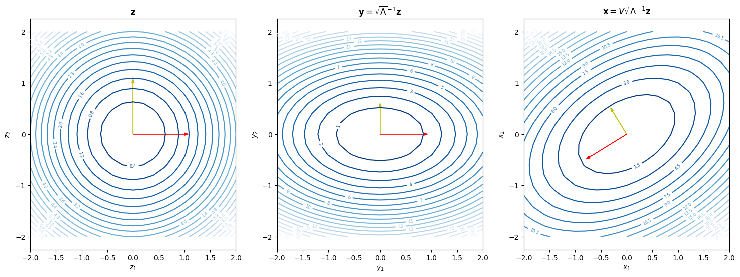

Note that countours of $f(\bfx)$ are exactly alinged with the transformed circle from $\bfz$ to $\bfx$

Eigen values of saddle point (Indefinite matrix)¶

A = np.array([[2, -1],
             [-1, -3]])
A

array([[ 2, -1],
       [-1, -3]])

lambdas, V = np.linalg.eigh(A)
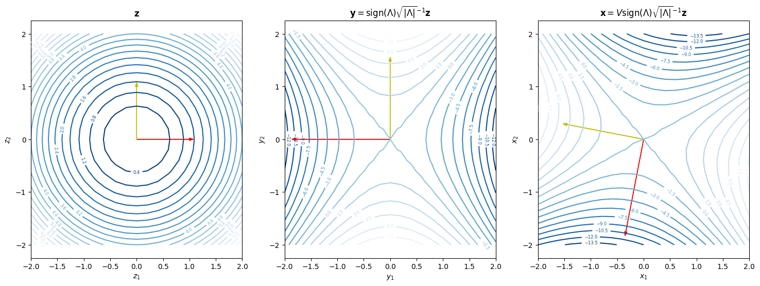
lambdas

array([-3.1925824, 2.1925824])

Note that the eigen values are neither all positive nor all negative. We cannot take the square root directly and we have to be respectful of the sign of the lambdas.

fig, axes = plt.subplots(1, 3, figsize=(18, 6))

ax = axes[0]
plot_contour(ax, f_wrt_z)
ax.set_title(r'$\mathbf{z}$')
ax.set_xlabel(r'$z_1$')
ax.set_ylabel(r'$z_2$')
draw_arrows(ax, zs)

ax = axes[1]
plot_contour(ax, partial(f_wrt_y, lambdas))
ax.set_title(r'$\mathbf{y} = \text{sign}(\Lambda)\sqrt{|\Lambda|}^{-1} \mathbf{z}$')
ax.set_xlabel(r'$y_1$')
ax.set_ylabel(r'$y_2$')
ys =  zs / np.sign(lambdas) * np.sqrt(np.abs(lambdas))
draw_arrows(ax, ys)

ax = axes[2]
plot_contour(ax, partial(f, A=A))
ax.set_title(r'$\mathbf{x} = V \text{sign}(\Lambda)\sqrt{|\Lambda|}^{-1} \mathbf{z}$')
ax.set_xlabel(r'$x_1$')
ax.set_ylabel(r'$x_2$')
xs = (V @ ys.T).T
draw_arrows(ax, xs)

<Axes: title={'center': '$\\mathbf{x} = V \\text{sign}(\\Lambda)\\sqrt{|\\Lambda|}^{-1} \\mathbf{z}$'}, xlabel='$x_1$', ylabel='$x_2$'>